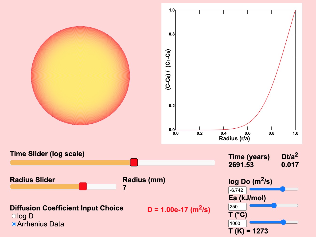
Figure 21. Diffusion in a Sphere. This diagram shows an exact solution to the diffusion equation given by Crank (1975, equation 6.18) for diffusion in a spherical isotropic mineral grain with the surface of the sphere held at a constant composition. Click on the image for a larger, interactive version where you can observe what happens as the model parameters are changed.
Move the time slider to 6760 years and the value of the parameter Dt/a2 should be 0.085 (with radius a = 5 mm and D = 1e-17 m2/s). Change the radius to 10 mm, then change the time to 27542 years. Once again, the parameter Dt/a2 should be 0.085 and the graph should look the same as it did before you changed the radius. Different values of the sphere radius (a), the diffusion coefficient (D), and the time (t) that yield the same value of Dt/a2 will have the same normalized composition profile.
Yes. If Dt/a2 > 0.6, even the center of the sphere will have a composition within 2% of the composition of the surface of the sphere (C1).
No. Reload Figure 21 and move the time slider unitl the spherical cross section on the left has changed from all yellow to all red. Try again.
Yes. If Dt/a2 > 0.6, even the center of the sphere will have a composition within 2% of the composition of the surface of the sphere (C1).
No. If Dt/a2 > 0.6, even the center of the sphere will have a composition within 2% of the composition of the surface of the sphere (C1).
Yes! Homogenization is proportional to the square of the sphere radius a. As we observed in Q1, homogenization requires Dt/a2 to be greater than 0.6. For simplicity, let Dt/a2 = 1. Then t = a2/D. If the value of a is reduced from 5 mm to 1 mm, t = 1/D rather than t = 25/D.
The sphere model is a good start for thinking about diffusion in an equant mineral grain such as olivine in a well-stirred magma. An example putting homogization by diffusion to use as a geochronometer is investigated in the next page.
No. Homogenization is proportional to the square of the sphere radius a. As we observed in Q1, homogenization requires Dt/a2 to be greater than 0.6. For simplicity, let Dt/a2 = 1. Then t = a2/D. If the value of a is reduced from 5 mm to 1 mm, t = 1/D rather than t = 25/D.
The sphere model is a good start for thinking about diffusion in an equant mineral grain such as olivine in a well-stirred magma. An example putting homogization by diffusion to use as a geochronometer is investigated in the next page.