Hofmeister's Rules - Dynamical System Model - Results

A Mathematical Model

We present the dynamical system model of phyllotaxis which has been the object of our research. It is a mathematical derivation of a model by the physicists Douady and Couder, which itself is based on observations by the 19th Century botanist Hofmeister. This model reproduces all spiral patterns exhibited by plants and explains why Fibonacci phyllotaxis is predominant. The applet Dynamical Model gives a simulation of this process.

Hofmeister's Rules

Return to Top

In 1868 the botanist Wilhelm Hofmeister published his microscopic study of meristems. He proposed that in spiral phyllotaxis, botanical units form one by one with the newest in the least crowded spot. Following Douady and Couder (1996, Part I), we make these rules a bit more precise:

• Primordia initiate one at a time in the least crowded spot around a circular meristem.
• Primordia are radially displaced away from the center as they grow.

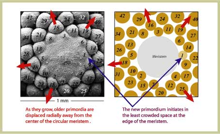
Compare a scanning electron micrograph of a Norway spruce (Picea abies) shoot apical meristem with a computer generated arrangement of primordia. The computer program implemented the mathematical model based on Hofmeister's rules and converged naturally to this configuration. Primordia are numbered according to their age - the higher the number, the older the primordium. Notice the remarkable similarity between plant and model.
Electron micrograph courtesy of Rolf Rutishauser, published in Rutishauser (1998).

Dynamical System Model

Return to Top

Our model is a discrete dynamical system. Generally, a discrete dynamical system consists of iterating a function (also called map) F on a set S (also called the state space). In this model, each element in S corresponds to a configuration of primordia, which are represented by points on concentric circles, with one point per circle. The innermost circle represents the periphery of the meristem. From circle to circle the radius increases by a constant factor G, that we call here expansion rate (Plastochrone ratio in the literature). Each configuration is encoded as a list of divergence angles between successive points. Hence, S can be seen as the set of all possible lists (d₁ , d₂ , . . . ,d_N) of angles.

Under the function F, points of a configuration move out radially to the next circle. The outermost point is eliminated and a new point (green) is generated on the innermost circle, where the distance to the closest point is maximum. The "distance-to-closest" function along the inner circle is represented as a graph (red).

the "distance-to-closest" function D(z), with variable z representing a point on the edge of the meristem is implemented as D(z) = min_k(dis(z, z_k)) where z_k is the point representing the center of primordium k. Clearly each z_k is function of the variable d₁ , d₂ , . . . ,d_N. The least crowded rule chooses the point z that maximizes D.

Results

Return to Top

Stationary points in Dynamical Systems The first feature that one usually studies in a dynamical system is its fixed, or stationary points. These are points in the state space which do not change under the map F. For example, the dynamical system given by squaring real numbers, f(x)=x² has fixed points 0 and 1, since f(0)=0 and f(1)=1. An important characteristic of fixed points is their stability. In the example of the squaring map, 0 is stable: if you start with a point close to 0 (e.g. 0.01), repeated squaring will only get you closer to 0. On the other hand, the fixed point 1 is unstable: repeated squaring of numbers greater than 1 will indefinitely increase these numbers, whereas repeated squaring of numbers smaller than 1 will decrease to 0; in either case, you will get farther and farther from 1. As a rule of thumb, if the dynamical system considered models a natural phenomenon, stable fixed points are significant in the sense that they can be perceived in experiments, as their stability allows for a margin of error in measurements.

Stationary configurations in the Phyllotaxis Model In the model F described above, we have the following results (see Hotton (1999) and Atela, Golé & Hotton (2002)):

• Stationary configurations of F are spiral lattices, i.e. configurations of constant divergence angles d₁ = d₂ = . . . =d_N (a trivial consequence of the rule of radial displacement).
• All stationary configurations of F are stable, accounting for the presence of spiral phyllotaxis in nature.
• Among all spiral lattices (each represented by a point of the disk below, see the Spiral Applet), those corresponding to stationary configurations form a collection of paths traversing regions of lattices with parastichy numbers following Fibonacci-like sequences. The two most prominent paths start, for large values of the expansion parameter G (represented by points closer to the center below), at the (1,1) (distichous) lattices (the red line segment starting leftward from the center), and follow regions of increasing Fibonacci numbers as G decreases.
  

A Scenario for Fibonacci Phyllotaxis These three results put together provide -given Hofmeister's rules- an explanation for the occurrence of spiral phyllotaxis in nature, as well as for the predominance of Fibonacci phyllotaxis in spiral phyllotaxis. Indeed, the expansion parameter G is known to decrease as plants grow, especially at the flowering stage. With large G the pattern has no choice but to converge toward a distichous phyllotaxis. As G decreases, and primordia are formed (i.e.. while the dynamical system is iterated), the stability of stationary configurations forces the nearby configurations to hover along one of the paths of fixed points which starts at distichous, that is, one of the two Fibonacci paths. As G decreases (moving away from the center in the picture), parastichy numbers increase along the Fibonacci sequence, and the divergence angle tend the Golden angle (upper path) or its complement (lower path). Such a scenario is numerically - and visually - verified in the Dynamical Model applet.

Hofmeister's Rules - Dynamical System Model - Results