Biological Sciences 300/301, Smith College | Neurophysiology
Lab 6: Electroretinogram of the Crayfish Eye
http://www.science.smith.edu/departments/NeuroSci/courses/bio330/labs/L6erg.html
Bio 300/301 Home | Schedule | Videos | Laboratories | Administrative Information
View the video: Electroretinogram of the Crayfish Eye.
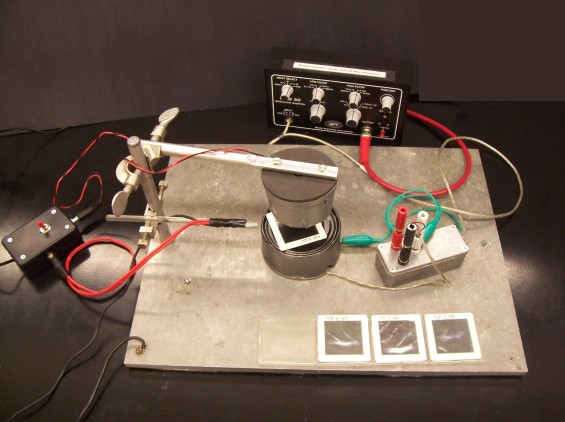
Equipment:
- Oscilloscope
- Chart recorder
- DAM-50 amplifier
- Recording chamber and shield
- Strobe stimulator
- Phototransistor for triggering
- Neutral density filters (0.2, 0.5, 1.0, 2.0)
- Dropping bottle with crayfish
saline.
1. Background.
The electroretinogram. Receptor cells typically respond to stimuli with prolonged, graded potentials. In some cases, the graded depolarization may initiate action potentials in the receptor cells. In other cases, the receptors make only graded potentials, but not spikes. Photoreceptor cells in the eyes of arthropods like the crayfish are generally of the non-spiking type. They respond to increased light-levels with increasing depolarization.
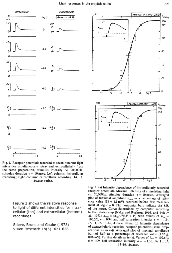
The electroretinogram, or ERG, is the synchronous response of many photoreceptors depolarizing together in response to a bright flash of light. The ERG is recorded with an extracellular electrode on or just below the surface of the eye, and a reference electrode elsewhere. As in other extracellular recordings, depolarization of the cells appears as a negative potential to the electrode outside the cells. A study that combined simultaneous intracellular and extracellular recordings from crayfish photoreceptors showed that the waveform of the extracellular ERG is a good representation of intracellular events in the photoreceptors. (In their figures, the ERG is plotted negative-upwards. We will follow the usual convention of negative-downwards in our experiment.)
Click images for enlarged views.
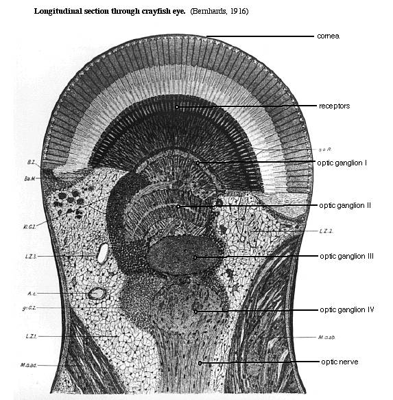
The crayfish eye. Arthropod compound eyes are composed of thousands of repeating units called ommatidia. Each ommatidium is a long tube with a cluster of photoreceptor cells at its base. Light enters the top of the tube to reach the photoreceptors. In dark-adapted eyes, some light also reaches the receptors in neighboring ommatidia. Axons from the photoreceptors go to the first of four optic ganglia in the eyestalk. The last optic ganglion sends axons in an optic nerve to the brain. In our experiment, we will place a pin electrode through the corneal surface, attempting to keep it above the receptor cells. In that way, we record the depolarization of the photoreceptors without also picking up responses from neurons in the optic ganglia.
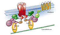
Second messengers. The ERG is also a good model system for metabotropic synapses. In the receptor cells, light activates second messengers that in turn open channels. Visual pigment molecules (rhodopsin) embedded in the photoreceptor cell membrane catch photons of light. Rhodopsin in turn activates a G-protein, which activates phospholipase C, which leads through several steps to the opening of a channel (the transient receptor protein, TRP). Ca++ and other small cations enter through the open channel and depolarize the receptor cells. Most of the steps in arthropod visual transduction have been worked out in Drosophila, but they are likely to be similar in crayfish.
In our experiments, we will see a lag of 10 or more milliseconds between the light flash and the start of depolarization. This lag is the time in which the second messenger system is activated and opens the TRP channels. Changing the brightness of the light will change the number of rhodopsin molecules that are activated, and thus the amount of second messenger that is produced. This is analogous to varying the amount of transmitter at a metabotropic synapse.
Neutral density filters. In our experiment, stimuli will be brief flashes of light generated by a strobe stimulator. The intensity of the light will be controlled by placing neutral density filters between the strobe stimulator and the eye. Neutral density filters appear gray (they are "neutral" in color) because they reduce the brightness of all visible wavelengths approximately equally. Each filter is marked with a number that gives its density, D, which is defined as:
D = log 1/T
where T is the transmittance of the filter. For example, if a filter transmits 1/10 of the light incident on it (1/10 transmittance), the filter's density is log 10 = 1.0. Similarly, if a filter transmits 1/100 of the light, its density is equal to log 100, or 2.0. The important point to notice is that a change of 1 in the density corresponds to a change by a factor of 10 in the light transmitted.
It is possible to measure the actual energy in a light stimulus, but in practice the relative intensity of the stimulus is often used. We will use relative intensity in our experiment. The brightest stimulus light (with no filters in the path) is given a relative intensity equal to 1.00. Dimmer lights will then have relative intensities between 1.00 and 0. Since an eye typically responds over a very wide intensity range, it is usually convenient to record the log of the relative intensity of the stimulus. The brightest light would have a log relative intensity of 0 (log 1.0 = 0), a light 1/10 as bright would have a log relative intensity of -1, and so forth. An especially convenient feature of using log relative intensity is that the density of the ND filters gives us the log relative intensity directly. The following table shows this:
|
ND filter (density) |
percent light transmitted |
log relative intensity |
|
0.0 (no filter) |
100% |
0 |
|
0.2 |
63% |
-0.2 |
|
0.5 |
32% |
-0.5 |
|
1.0 |
10% |
-1.0 |
|
2.0 |
1% |
-2.0 |
|
3.0 |
0.1% |
-3.0 |
A final point: ND filters can be stacked up, in which case the density of the combined filters is equal to the sum of the densities of each component. For example, a 1.0 filter and a 2.0 filter stacked together equal a 3.0 filter.
You can work this out intuitively as follows: the 1.0 filter lets through 1/10 of the incident light, and then 1/100 of that 1/10 is allowed through the 2.0 filter. Both filters together allow through 1/10 x 1/100 = 1/1000 (0.1%) of the incident light. This is the same amount that is transmitted by a 3.0 filter.
View the video: Electroretinogram of the Crayfish Eye
2. Experimental procedure.
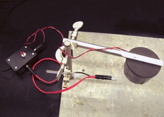
Strobe stimulator. A strobe light provides a very bright, very brief flash that makes a convenient visual stimulus. Clamp the strobe above the tin-can shield that will cover the eye-holder, leaving enough room to insert several filters between the strobe and the shield. Plug the strobe's power cable into the switched outlet on the short side of the 12-volt power box.
To trigger the oscilloscope each time a flash occurs, we will use a phototransistor, a semiconductor whose resistance decreases in the light. The phototransistor has been wired in series to a resistor and voltage source so that each light flash produces a voltage pulse. Clamp the phototransistor to point to the side of the shield. (Since the flash is so bright, it can saturate the transistor and give a distorted record if the transistor faces the strobe directly.) Connect the phototransistor's red power cable to the unswitched outlet on the long side of the 12-volt power box. Connect the black signal cable to the patch panel for channel 2 of the oscilloscope.
Set up the oscilloscope. Make sure that CH1 and CH2 are both on, and that two traces appear on the screen. Use DC coupling for channel 1 (the ERG) and AC coupling for channel 2 (the strobe pulse). Set the vertical scale for CH2 at its least sensitive setting (5 V). You can later adjust it to be more sensitive (2 V or 1 V per division) if necessary.
Turn on the strobe. In the Trigger menu, select:
- Source: CH2
- Sweep: Normal (not Auto)
Adjust the trigger level knob until each strobe flash triggers a sweep.
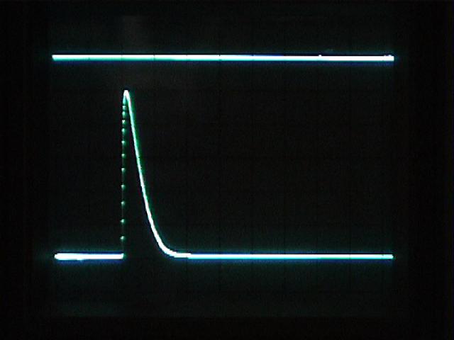
Before you do the main experiment, take a minute to examine the strobe pulse. Stretch out the oscilloscope's time scale enough to see the shape of the pulse. If the top of the pulse is flat, the signal is being clipped. Move the phototransistor farther away from the strobe light, or cover the transistor with a small bit of white paper until the strobe pulse has a non-flat top. Capture a screenshot on your USB flashdrive. From the screen, measure and write down the strobe pulse's width (in units of time) at half-amplitude (halfway between its peak and the baseline).
Later, when you have slowed the sweep to see the ERG, you will find it interesting to compare the very brief duration of the strobe flash to the much longer latency and duration of the ERG.
Prepare the main experiment. Connect the output of the DAM-50 amplifier to channel 1 on the patch panel. Set the amplifier for differential recording (A-B), the mode to AC, and the low-frequency filter to one of its lowest settings. Set the oscilloscope's input coupling for channel 1 to DC (CH1 menu) if you have not done so already. These settings will minimize distortion of the relatively slow ERG.
Since the eye will not last indefinitely, plan to do all the experiments in one quick sweep. Plot graphs and make calculations afterward.
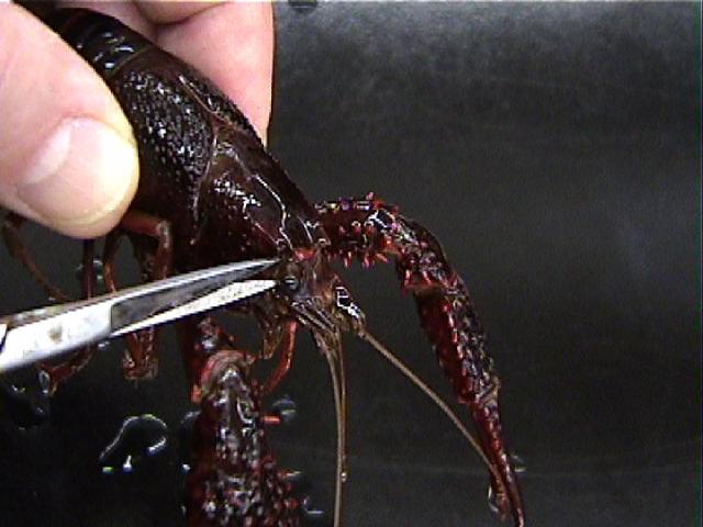
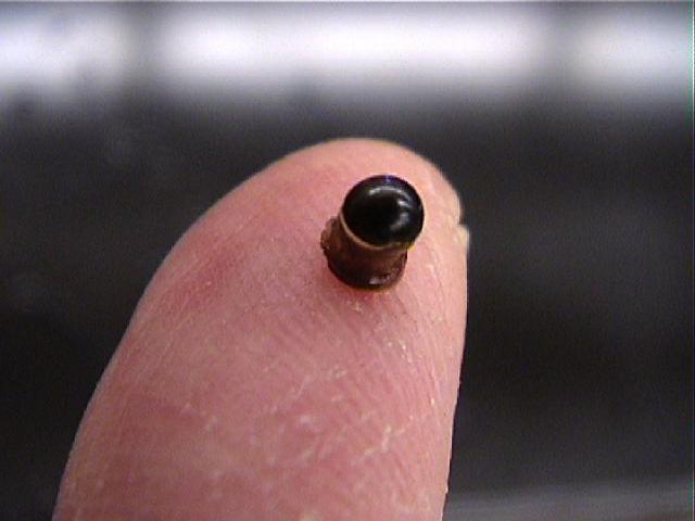
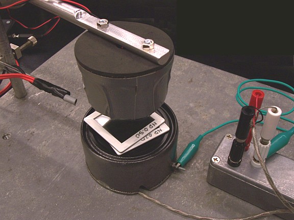
Dissection. Cut the eye from a crayfish at the base of the eyestalk. If possible, use a crayfish whose other eye has already been removed. You will be able to see where to make this cut more easily if you first cut off the pointed rostrum that partially shields the eyes.
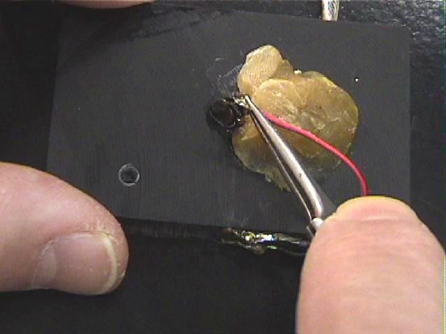
Place a drop of crayfish saline into the well of the recording chamber. Insert the base of the eyestalk into the well. There are two electrodes in the well: one is a ground, and the other is the reference electrode. Advance the needle electrode toward the cornea of the eye until it punctures the cornea. Place the recording chamber under the strobe and cover it with the tin-can light shield, which you should ground with a clip-lead. Plug in the electrodes and check for 60-Hz noise. If all is well, you will not need to touch the eye or electrodes for the rest of the experiment. If there is a lot of 60-Hz noise or too much baseline drift (even after increasing the low-frequency filtering), check that the needle electrode is actually puncturing the eye.
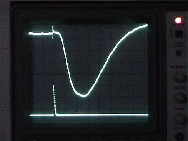
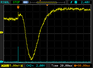
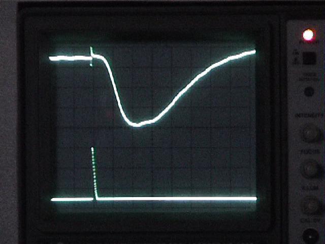
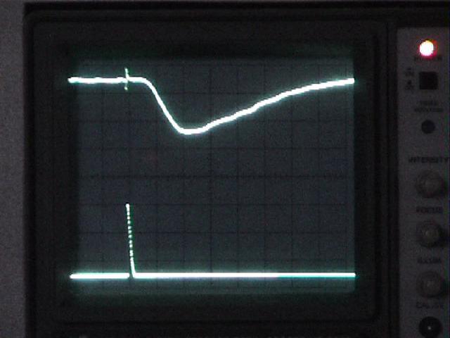
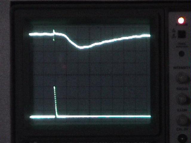
Top trace: ERG
Bottom trace: strobe pulse
Time course and amplitude of the ERG.
Adjust the oscilloscope's horizontal scale and vertical sensitivity for CH1 until the ERG fills the screen. You may wish to move the trigger point closer to the left edge of the screen.
Note: reduce the fast sweep speed that you used to examine the strobe's response, or you will see only the strobe artifact and miss the much slower ERG, which occurs tens of msecs later.
If the ERG trace is very "fat," adjust the amplifier's high-frequency filter setting to filter out noise. The 1 kHz setting should be adequate, but see if the other high-frequency filter settings improve the signal. Adjust the amplifier's low-frequency filter to eliminate baseline drift without unduly reducing the amplitude of the ERG.
 Capture
screenshots of one or two good examples of the
ERG. Write down the following measurements:
Capture
screenshots of one or two good examples of the
ERG. Write down the following measurements:
- the amplitude of the response from baseline to peak, at the electrodes (divide the ERG's apparent amplitude on the screen by the amplifier's gain).
- the latency of the response (the time, in msec, from the start of the flash to the initial phase of the response). Estimate the latency along the baseline, but since it is difficult to determine exactly when the ERG starts, also measure from the stimulus to the "half-amplitude" point, halfway between the baseline and the peak. Use this half-amplitude latency when you make intensity-response measurements (next section).
- also measure the duration of your examples, both at the baseline (a good estimate of the total length of time the depolarization lasts) and at the half-amplitude level (an easier measurement to make accurately).
In the next section, you will measure ERG amplitude and half-amplitude latency for different light intensities, but you do not need to measure the durations each time.
Intensity vs. response. [Note that you will need to do this series twice, once working from bright to dim stimuli, and then working back from dim to bright. This will help correct for dark adaptation or any other changes in the eye's responsiveness during the measurements.]
Place a series of neutral density filters on top of the tin-can shield (interposed between the strobe light and the eye) while you write down the ERG amplitude (from the baseline before the strobe artifact to the peak of the response) and the half-amplitude latency.
- Work from bright lights (no filters) to dim lights
(dark filters) in one quick sweep, and then repeat the
measurements in reverse (dark filters to no
filters).
- Use a combination of filters in a systematic
progression: 0 (no filter), 0.2, 0.5, 0.7 (=0.2 + 0.5),
1.0, 1.2, etc. Stop adding filters when you can no longer
resolve the response against the noise of the
baseline.
- For small responses, increase the oscilloscope's
vertical sensitivity to measure the response accurately.
Keep track of the vertical scale when you make these
measurements.
- Use Averaging
of 8 or 16 traces [Acquire menu] to pull a
weak signal out of noise.
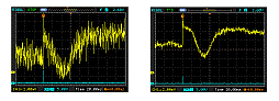
An example of signal averaging, where a noisy response to a dim flash (left) is "cleaned up" by averaging repeated responses to the flash (right). A supplemental page explains how to set up signal averaging.
- Keep the light source at a constant distance from the preparation. The light intensity is proportional to the inverse square of the distance between the source and the target, and the intensity will change if the distance is changed.
Collect your data in a written table that shows the value of the neutral filters, the ERG amplitude (both the volts on the screen and the equivalent volts at the electrode, after correction for the amplifier's gain), and the half-amplitude latency from the flash to the response.
(Optional) After you have collected your data, you may wish to capture screenshots of a few representative responses to different stimulus intensities.
Demonstrating responses to prolonged light pulses
and to brief pulses repeated at high rates (flicker fusion).
For this part of the experiment, we will replace the strobe stimulators with
bright LEDs driven by our Grass stimulators. Although it is difficult to
calibrate the brightness of the LEDs for different stimulator voltages, it
is easy to set the LED to a single high brightness, and then vary the duration of the
light pulses to see how the ERG responds to a pulses of hundreds of msec
rather than the fraction of a msec that the strobe provides. It is also possible
to repeat very brief flashes at high rates to determine when the ERG no longer
detects the flashes as separate events, instead fusing them into a steady
response. This is the "flicker fusion frequency," which for people is between 60
and 90 flashes/second. [A practical consequence of the human flicker fusion frequency
is reflected in cinema technology. Movies are recorded at 24 frames per second,
which would flicker, but when they are projected, each frame is presented two or
three times by a rotating shutter to produce 48 or 72 images/sec. This is
above the human flicker fusion frequency (data from Wikipedia).]
Preliminary check of the LED's output: Connect the LED's wires to the stimulator's output, and the stimulator's synch pulse to the oscilloscope's external trigger. Examine repeated flashes from the LED while varying the pulse duration and the output voltage, watching the LED's light to find a setting that produces consistent bright flashes. Then monitor the LED output with the same phototransistor you used to detect strobe flashes, checking to see if the LED's brightness varies for different pulse durations and repetition rates.
Experiment 1: Record the ERG for [infrequent] long-duration pulses. Does the depolarization decrease to a plateau after the initial response?
Experiment 2: Determine the flicker fusion frequency by presenting very brief flashes (1 or 2 msec duration) at increasingly high rates until the ERG no longer shows separate responses to each flash. (Does the flash duration affect the flicker fusion frequency?)
For the final experiment, you can again use the strobe stimulator, or you can try using the LED, presenting brief pulses repeated at a moderate rate (similar to the strobe flashes).
Demonstration of dark- and light-adaptation. Most of us have had the experience of entering a dark movie theater after being in daylight, and at first seeing nothing, but after a few minutes being able to see the people in the room. This is an example of being light-adapted initially, and then becoming dark-adapted with time in the dark. We have also had the opposite experience of being indoors in relatively dim light and emerging into a bright sunny day; initially we feel blinded, but we eventually become more comfortable with the bright outdoor light. This is an example of light-adaptation. We can easily demonstrate dark- and light-adaptation in the ERG.
NOTE: Although this section describes using your chart recorder to capture light and dark adaptation, you can use LabChart in addition to or instead of the EasyGraf recorders. (LabChart will give you more flexibility in displaying and analyzing the responses.) The following instructions are for the chart recorders, but you can create equivalent settings in LabChart.
Prepare to write the ERG directly to your EasyGraf chart recorder by connecting the chart-recorder's input cables to the patch panel to pick up the output of the amplifier (channel 1) and the strobe pulse (channel 2). Make sure both chart channels are on by pushing in their position controls. Adjust the chart's gain controls so the two signals are displayed appropriately. You can use the green readout to help you position the two traces on the chart and to set their gain appropriately. You want the ERG's baseline to be positioned near one edge, and the ERG amplitude to be large enough to be seen easily and measured. You can check the settings by running the chart briefly, making any adjustments that are needed. Also make sure that the chart's annotation, grid and time markers are on, which will make it easier to make measurements.
To record the demonstration, run the chart at a slow speed (1 mm/sec). Turn on the strobe, and keep the strobe and the chart recorder running for the entire demonstration, even when the eye is not receiving the flashes. The chart will give you a time record for the entire experiment.
Make sure you understand the relationship between the appearance of the ERG at a compressed time scale and the oscilloscope's display -- you want to measure the ERG but not the artifact from the strobe flash. Temporarily run the chart at a high speed (25 or 50 mm/sec) for two or three flashes. This will help you interpret the compressed record (at 1 mm/sec) by showing you the shape of the ERG on the chart record when time is more stretched out.
Establish a baseline recording of the responses for at least one minute of strobe flashes (no filters). The eye has been sitting in semi-darkness during the prior measurements, and its responses should be relatively dark-adaptated. To check if the strobe flashes themselves slightly light-adapt the eye, cover the opening in the shield with an opaque square of cardboard. (The chart should be left running.) After one minute, remove the opaque square and observe the responses on the chart. If the eye has dark-adapted during the minute of complete darkness, the first responses will be bigger than the prior baseline responses. Allow the responses to reach a new plateau level, which will be the baseline amplitude for the next measurement.
Without changing the strobe's height, position the fiber-optics light pipe (from your microscope illuminator) to point through the opening of the shield at the eye. Turn on the light to light-adapt the eye. After 30 seconds, remove the light pipe and re-position the strobe as it was before Are the initial responses smaller, indicating light-adaptation? Does the eye dark-adapt again? The responses may increase to a new plateau, usually smaller than before. Once a plateau amplitude is reached, stop the experiment.
Measure and make a table showing the amplitude of responses before dark- and light-adaptation (you can estimate the average level), the amplitude of the first response just after adaptation, the new plateau level, and the time it took to reach the new plateau. In your table, express the amplitudes as their absolute values and also as the percent of the baseline amplitude for that portion of the experiment.
3. Plot your data.
Before you leave lab, upload several files to your team's Drive folder:
(1) a good screenshot of the ERG. Also include a table of the measurements you made of the ERG's amplitude at the electrodes, the latency, and the duration. You may (optionally) include several representative screenshots of the ERG for different stimulus intensities.
(2) a graph plotting the relative stimulus intensity (ND filter values) against the ERG's amplitude and latency. You can download a PDF file of 1/8-inch graph paper to use for plotting:
- the two measurements (bright-to dim-stimuli,
and the reversed order of dim-to-bright) of the
amplitude of the ERG ( in mV or µV at the
electrode) for each intensity, and their
average;
- on the same graph, the half-amplitude latency
between the flash and the ERG, using another vertical
axis and different symbols to indicate latency in msec.
NOTE: It is customary to plot the stimulus intensity on the horizontal axis, and to place the dimmest stimulus (the darkest filter, ND=3) at the left, and the brightest stimulus (ND=0) at the right.
(3) A table of dark- and light-adaptation responses.
4. Clean up.
At the end of the afternoon,
- Rinse the eye-chamber in tap water, and clean and dry your dissection tools.
- Copy files from your thumb drive to a folder on your computer, and erase the thumb drive for the next group's use.
- Move any files and folders on your computer's desktop into your own group's data folder.
- Turn off all equipment, including the DAM-50 amplifiers.
Revised March 15, 2021.
Back to laboratory table of contents page
Using Gould EasyGraf Chart Recorders
© 2003, 2011 by Richard F. Olivo. Permission is granted to non-profit educational institutions to reproduce or adapt this Web page for internal use provided that the original source and copyright are acknowledged.