
Biological Sciences 330, Smith College | Research in Cellular Neurophysiology
Motor Units in the Crayfish Nerve Cord
Revised: February 28, 2019
Knowing of my growing curiosity about
invertebrate animals, particularly about the crayfish,
[Harry] Grundfest suggested that I set up an
electrophysiological recording system with Crain's help.
I could use the system to replicate Hodgkin and Huxley's
experiment by recording from the large axon of the
crayfish, which controls the animal's tail and thus its
escape from predators. This crayfish axon is smaller than
that of the squid but nonetheless very large.
Crain showed me how to manufacture glass microelectrodes for insertion into individual axons and how to obtain and interpret electrical recordings from them. It was in the course of those experiments -- which were almost laboratory exercises, since I was not exploring new ground scientifically or conceptually -- that I first began to feel the excitement of working on my own. I connected the output from the amplifier I was using to record the electrical signal to a loudspeaker, as Adrian had done thirty years earlier. Whenever I penetrated a cell, I, too, could hear the crack of an action potential. I am not fond of the sound of gunshots, but I found the bang! bang! bang! of action potentials intoxicating. The idea that I had successfully impaled an axon and was actually listening in on the brain of the crayfish as it conveyed messages seemed marvelously intimate. I was becoming a true psychoanalyst: I was listening to the deep, hidden thoughts of my crayfish!
Eric Kandel, In Search of Memory (NY: WW Norton & Company, 2006) pp 108-109.
Supplement: Anatomy of the Crayfish Nervous System.
This afternoon's lab has two sections: a review of the detailed neuroanatomy of the crayfish nerve cord (for which you should allocate about 30 minutes), and a physiological experiment (the main part of today's work).
Click images
for
larger versions.
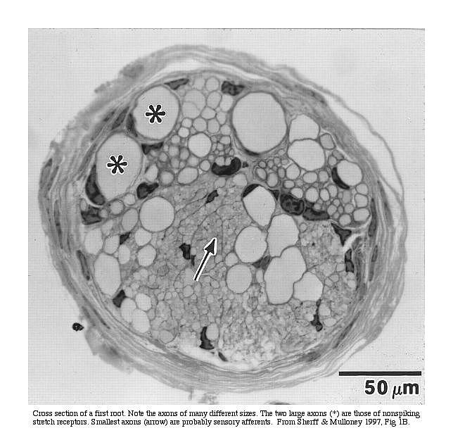 Cross-section
of root 1. Note the different sizes of axons (circular
profiles) in the root. Source: Sherff and Mulloney
(1997).
Cross-section
of root 1. Note the different sizes of axons (circular
profiles) in the root. Source: Sherff and Mulloney
(1997).
See the Supplement
on crayfish neuroanatomy.
A. Neuroanatomy
1. The crayfish nerve cord.
The material below reviews the main functional aspects of the abdominal nerve cord. After you have read it, you and your partners will work with digitized serial sections of a ganglion to find major structures.
The crayfish abdominal nerve cord has been widely investigated because of its relative simplicity. The cord consists of six ganglia (AB1 to AB6 in the figure) joined by connectives. From each ganglion, three bilateral (left & right) pairs of nerves ("roots") innervate the muscles and sensory receptors in that abdominal segment. (The sixth ganglion, nearest the uropods and telson, is a fusion of two embryonic ganglia.) Each of the three roots has a different destination in its segment of the abdomen, as described below. In our physiological experiment today, we will record from whichever of the roots gives the best recording. The motoneurons are tonically active, generating spontaneous spikes that we will listen to as well as watch. This tonic motor activity produces a continuous low level of muscle tension which keeps the joints of the abdomen stiff.
The first roots innervate the swimmerets. The roots branch to innervate separately the muscles driving forward and backward motions of the swimmerets. In an intact animal, the swimmerets often beat rhythmically for periods of many seconds, with the beat frequency typically about 1.4 beats/second. The rhythmic motor activity is produced by pattern generator circuitry in each abdominal ganglion. The rhythm sometimes appears spontaneously in a fresh preparation, or it can be evoked pharmacologically. The figure below shows the swimmeret motor pattern recorded from the return-stroke (RS) and power-stroke (PS) branches of the first root.
|
|
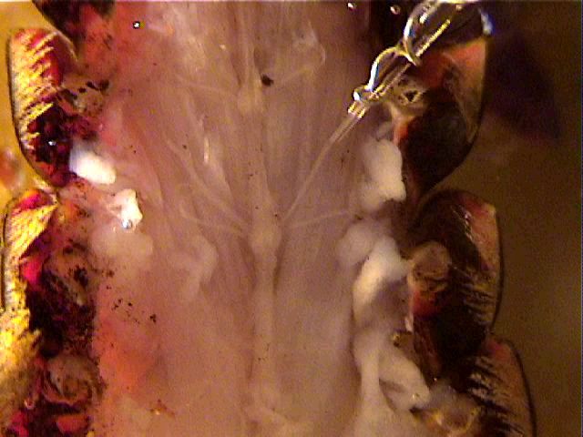
Recordings from the anterior and
posterior branches of a first root (N1), showing
alternating bursts of activity in axons from the
return-stroke (RS) and power-stroke (PS)
motoneurons. |
The second roots innervate the extensor muscles of the abdomen. There are thirteen motor axons in each root, six to the superficial extensor muscles, and six to the deep extensor muscles. The thirteenth motor axon goes to the stretch receptor sensory cells. (The second root also carries sensory axons from tactile hairs and the stretch receptors, but those axons will be silent since we will cut the connection to the periphery.) Since there is such a small number of motor axons in a second root, and since the root is the easiest to record from because of its size and position, the second root will probably offer the best opportunity for following the activity of single motoneurons.
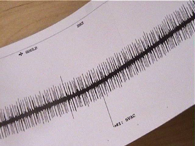
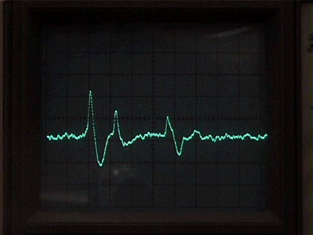
Spontaneous motor unit activity recorded with a suction electrode on the second root of a crayfish abdominal ganglion. Spikes of different sizes represent different motor axons. Source: class experiment by Jill McCullough and Lizette Pabon.
The third roots leave the connective a short distance posterior to each ganglion, and dive into the underlying muscle. They are strictly motor, and innervate the deep and superficial flexor muscles. Each third root contains 16 motor axons: 10 of these are large axons and supply the fast flexors (9 excitors and one inhibitor axon).The other six are smaller axons that supply the slow flexor muscles (5 excitors and one inhibitor). The motor neurons that send axons to the third root were among the first neurons to be uniquely identified and have their geometry mapped through intracellular staining with Procion yellow.
The third root provides a good example of being able to follow the firing of individual neurons in a multi-unit recording. The six axons supplying the slow flexor muscles on one side of a segment are all packaged together in the third root's superficial branch. In extracellular recordings, the action potentials of the six axons can be distinguished on the basis of spike size. For example, the record below shows spontaneous activity recorded simultaneously from the superficial branch in segments 2, 3, and 4. One can see at least five different spike sizes in the record from segment 3. Each spike size represents a different axon's activity; thus we can follow the firing of five different motor neurons in this record. A goal in lab today is to obtain records similar to this figure from any of the roots
|
|
Spontaneous motor activity in the superficial branch of the third roots from ganglia 2, 3, and 4. Time marker: 100 msec. |
2. Digital neuroanatomy: serial sections of an abdominal ganglion.
Launch the supplement on the Anatomy of the Crayfish Nervous System with its figures of stained neurons and spectacular videos showing sequential serial sections through a ganglion. With your lab partner(s), first look at the six still images under "Stained swimmeret motoneurons" at the bottom of the page. These pictures are of motoneurons whose axons exit in the first roots, innervating the swimmeret muscles. They were obtained by backfilling the first root to find the cell bodies of neurons whose axons are bundled in that root.
|
The positions of the motoneurons serving all three roots have been determined by backfilling. There are about 200 motoneurons in each ganglion. The adjoining diagram shows the cell bodies of the motoneurons sending axons out roots on the left side: 70 to the swimmerets (1st root), 13 to the extensor muscles (2nd root), and 17 to the flexor muscles (3rd root). |
|
(Click the figure for a larger image.) Source: Mulloney & Hall (2000) J Comp. Neurol. 419: 233-243.
Next, work with the "Videos of serial sections" that show all of the neurons and axon bundles in an abdominal ganglion.
|
First, orient yourself to the small drawing that shows the plane of section for Transverse, Sagittal, and Frontal sections. (Frontal sections are parallel to the plane of the screen.) Then view each of the three videos, looking for these major landmarks: |
|
- the regions where the first and second roots (N1 and N2) leave the ganglion
- the four giant axons that run from anterior to posterior near the dorsal surface of the nerve cord
- major tracts and left-right commissures of axons that cross the ganglion
- regions of neuropil (synaptic connections) in the center of the ganglion
- the locations and relative sizes of cell bodies of motoneurons and interneurons along the ventral surface of the ganglion
- profiles of axons in the connectives and roots
(note the range of diameters).
NOTE that after the video has played, you can drag the slider (the circle) or use the arrow keys to move through the sections individually.
After you have looked closely at all three series of sections, select one frame that shows details of a first or second root (the third roots are not in these sections because they exit from the connective posterior to the ganglion). Capture a computer screenshot of this frame to include in the material you post at the end of lab.
B. Physiology
3. Equipment
|
|
|
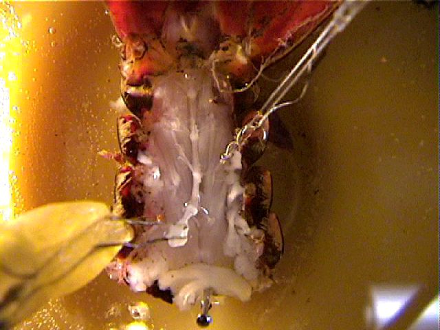
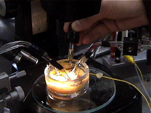
We will use suction electrodes in recording from the roots. The advantage of suction electrodes is that the preparation can remain immersed in saline; it is not necessary to lift the nerve branch into air. Instead, the nerve to be recorded from is cut, and the cut end is sucked into the electrode. The electrode must fit the nerve tightly to produce a good recording. After placing the electrode, our goals today will be:
- to observe spontaneous single-unit activity in one or more motor nerves and obtain screenshots, chart records, and computer files; this is the main part of the experiment.
- (optional) to stimulate activity electrically; and
- to observe the responses to a neuroactive drug (nicotine) that mimics ACh and elicits a long burst of spikes.
As an optional exercise, in addition to observing spontaneous activity, we can electrically stimulate motoneurons to increase their firing. In each ganglion, the motoneurons receive synaptic inputs from interneurons, many of which run the length of the nerve cord and excite groups of motoneurons in each segment. We can drive some of these interneurons by stimulating the anterior end of the cord. This will evoke firing in the postsynaptic motoneurons whose axons we monitor in the roots.
To interpret what we see at the recording electrode, it is necessary to understand that there are several types of pathways between the stimulating and recording points. The second root, for example, carries sensory axons that enter the ganglion and continue directly up the nerve cord toward the brain. Electrical stimulation of a connective creates antidromic ("backwards travelling") action potentials in these "straight-through" axons. The antidromic action potentials appear at the recording electrode with very little "jitter," since there are no intervening synapses. The electrical stimulus also excites interneurons that synapse (directly or through one or more intervening neurons) on motoneurons and excite action potentials. Because of the intervening synapse(s), the action potentials in postsynaptic units have a variable delay, and may drop out completely at high rates of stimulation. Both "straight-through" and postsynaptic units are seen in the accompanying illustration.
|
|
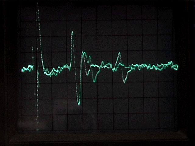
Multiple exposure of firing in a crayfish second root during repetitive stimulation of the connective. The stimulus artifact appears at the left of the trace. |
Displaying spontaneous neural activity: oscilloscope screens, chart records, and computer files.
One goal of today's lab is to become adept at displaying extracellular neural activity using three different technologies: oscilloscopes, chart recorders, and computer files.
A. Our digital storage oscilloscopes can display extracellular spikes at both fast and slow sweep speeds. At fast sweep speeds, it will be easy to see the size and shape of individual spikes.
At slow sweep speeds (horizontal scale settings of 100 ms/div or slower), the overall pattern of spike activity can be observed. For this to work well, the PeakDetect setting must be selected in the Acquire menu. This setting guarantees that the most positive and the most negative samples for each spike are displayed rather than a sample at some random point within a spike's waveform.
When a slow sweep is stopped (Run/Stop button), the horizontal scale and position knobs can be used to expand the scale and scroll through the entire record to inspect individual spikes. The position of the current screen within the overall record is shown by the zig-zag line at the top of the display.
B. The EasyGraph chart recorders can write extended examples of extracellular spikes on a long strip of chart paper for measurement and analysis. Direct writing works well because the EasyGraph recorders use an algorithm similar to the PeakDetect setting on our digital oscilloscopes. They sample the input signal at a high rate and draw a vertical line between the minimum and maximum sampled voltages for each column of dots. This displays spikes well.
To prepare for chart recording, connect the chart recorder's input cable for channel 1 to the output of the preamplifier at the patch panel. Push in channel 1's position knob to turn the channel on. Pull channel 2's knob out to turn that channel off. Center channel 1's trace, using the green dot display. To reduce baseline drift, set channel 1's input (on the chart recorder) to AC-coupling. Set the date and time if necessary. Make sure you have turned on the timer and enabled annotation.
You may also prefer to turn off the grid so that spikes are easier to see. Time marks at the bottom of the chart (seconds and larger 10-second tics) will let you measure time even with the grid off. Run the chart briefly at 10 mm/sec to make these adjustments.
C. PowerLab data acquisition system. In addition to acquiring chart records of activity, our computers can record long digital files of activity for display later. We will use PowerLab hardware and LabChart software (ADInstruments) to digitize and display the neural activity.
Connect BNC cables between the patch panel and the inputs to channels 1 and 2 on the PowerLab input box. For today, this will bring channel one's signal to the computer for digitization, with channel 2 connected but unused. See the appendix Capturing Data with PowerLab and LabChart for the initial steps in preparing to record computer files. (You will have to wait to set the "input range" (vertical scale) until you have made the dissection, placed the electrode, and are detecting spikes.)
View the video: Motor Units in Crayfish Abdominal Ganglia.
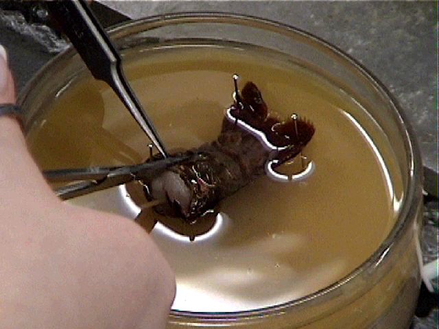
4. Dissection, and placing the electrodes.
Begin the disssection by obtaining a crayfish and chilling it in an ice-water mixture to slow its movements to a rate you find acceptable (there is no effective way to pith a crayfish). Cut off the abdomen ("tail") as close to the thorax as possible. Pin the abdomen ventral side up in a deep dissecting dish and add crayfish saline to cover it.
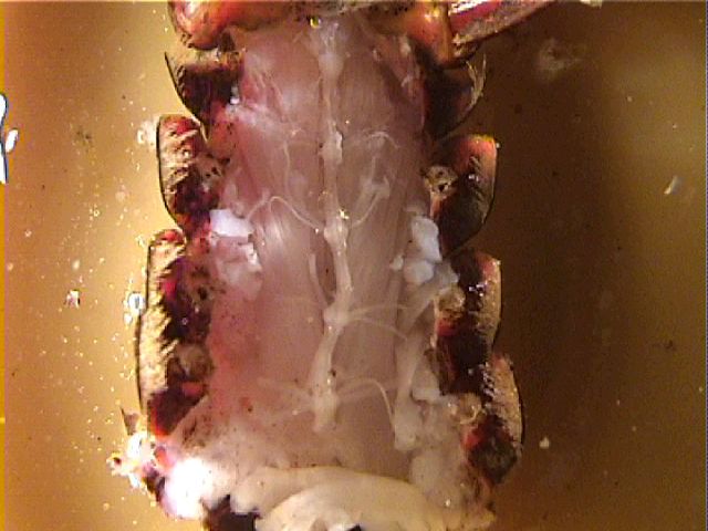
Starting at the cut end of the abdomen, make a long incision parallel to the midline but well over toward the side on which you will position the suction electrode. Use caution because the ventral nerve cord lies just below the exoskeleton. (However, if you accidentally cut the nerve roots on one side, it is not a problem. You will want to cut some of them anyway to pick up with the suction electrode.) Extend the incision almost to the tail fan. Lift the exoskeleton cautiously, peeking under it to make sure that the nerve cord is not adhering to it (if it does adhere, gently scrape it free with a scalpel). Cut away the flap of exoskeleton to expose the nerve cord and ganglia in the first four segments. If possible, keep the nerve roots intact on the side opposite to your first cut.
Locate all three roots of the third or fourth abdominal ganglion. (The third root, which leaves the connective posterior to the ganglion and dives into the muscle, can be found by gently sliding a glass probe under the connective.) If the roots were not already cut by your first incision, cut them on one side as far as possible from the ganglion. The piece of each root still attached to the ganglion will be picked up in a suction electrode.
In preparation for recording, ground the saline of the bath by attaching a clip lead between a ground point and a small length of silver wire that is dunked in the bath and fastened with tackiwax to the lip of the dish. Do not immerse the clip itself or you will get an unstable baseline.
Mount a suction electrode in the manipulator, and position the electrode so its tip will be able to reach each of the three roots that you have dissected. Lower the suction electrode into the saline and draw a little saline into the tip. Eliminate any air bubbles that lie between the tip and the internal wire (they would prevent electrical contact between the nerve and the wire). Position the tip of the electrode so that it touches the cut end of a root, and gently draw the end of the root into the suction electrode. If the nerve fits very loosely, fold it into the electrode by placing the electrode tip a few mm from the cut end and drawing that region in first.
5. Experimental procedure.
Try recording from each of the three roots that you have dissected. When you have discovered which root gives you the best recording, do the rest of the experiment on that root.
Observe spontaneous neural activity in the root. Can you distinguish individual motoneurons, based on spike size? Attempt to follow the firing of the largest and most active motoneurons by triggering the oscilloscope on their spikes. Explore whether you can increase the firing rate of any units by touching the uropods or telson, or by gently moving the swimmerets. Is there any evidence of reflex connections between sensory receptors and the motoneurons? If you are working with the first root and the swimmeret motor rhythm is present, try to get a chart record of it (the probability of finding the spontaneous rhythm goes down sharply as the preparation ages).
Then record samples of the activity for plotting and analysis:
A. Capture records of spontaneous tonic activity in a root using three different methods:
- Oscilloscope: Select PeakDetect in the
Acquire menu if you have not already done so. Observe the
spikes at both fast and slow sweep speeds. At fast sweep
speeds, triggering on the spikes will place one spike at
the trigger point on each sweep, with spikes in other
axons occuring at random times before and after this
point. Trigger the sweep on a large spike and capture
oscilloscope screenshots of that spike and other
spikes that appear in the same sweep. Calculate the true
vertical sensitivity as µV at the electrode,
after you correct for the DAM-50 preamplifier's gain.
Also observe activity at slow sweep speeds. Make sure the trigger point is near the left edge of the screen, or you will have to wait for samples to be collected up to the trigger point before the sweep is plotted. Stop the sweep with the Run/Stop button, and use the horizontal scale and position knobs to expand the time scale and move through the collected data. (Remember to restore the initial scale and trigger point when you return to live display.)
Select your best fast and slow screenshots to include with your other results.
- Chart recorder: Plot some spontaneous activity
on your chart recorder. Center the trace and adjust the
channel's gain (full-scale voltage) to make the spikes
big enough to be seen easily. You
will be able to read time directly from the chart
annotation, and the full-scale voltage setting
will tell you the vertical sensitivity (after correction
for preamplification). Your estimate of the peak-to-peak
amplitude of the largest spikes should be the same as
your measurements from the oscilloscope screen, since
both instruments are looking at the same activity from
the preamplifier. (If you get significantly different
estimates, check that you are reading the scales
correctly, or ask for help.)
Try different chart speeds to examine different resolutions and levels of detail (10 mm/sec is a good speed to start with).
- Computer: Use your PowerLab system and LabChart software to capture one or more examples of spontaneous firing as computer file(s). (See the appendix: Capturing Data with PowerLab and LabChart.) On your computer screen, expand LabChart's timescale and scroll through the captured record to visualize individual spikes. Use the Spike Histogram module to isolate a single spike and plot its firing pattern.
B. Estimate the average firing rate of a single axon using two methods:
- On a chart record, identify several of the largest
units (spikes in different motor axons) and put numbers
above them to mark when each unit fires (1= largest spike,
2= next largest, etc.). Calculate the average firing rate
(spikes/sec) of the most active unit(s) during a 10 to
20-second sample.
- Using Chart's Spike Histogram module, isolate a single
spike and plot the discriminator's output on a second channel. Use
the Frequency function (Cyclic Variables) to display the instantaneous
firing rate on a third channel. Estimate the average firing rate from the
plotted frequency and compare it to the value you calculated from the paper
chart record in the previous section.
When you have finished this section, save the file and open a new window to collect the data for the nicotine experiment. In the new window, display only one channel (to show the raw data), without any additional channels for calculations.
Electrical stimulation
(optional). Free enough of the anterior end of the
nerve cord to be able to lift that end of the cord above the
saline. Clamp hook electrodes in a small manipulator, lower
the electrodes into the saline next to the cord, gently ease
the cord onto the hooks (a glass probe can be useful here),
and raise the hooks (and the end of the cord) out of the
saline. Attach the hook electrodes to the output of your
stimulator. Stimulate interneurons in the cord by
gradually increasing the stimulus voltage. Trigger the
oscilloscope from the stimulator's "prepulse" output.
Stimulate at low rates (eg, 1-10/sec), and look for
responses in the root that are locked to the
stimulus. If you find a response, also try stimulating at
fast rates. As mentioned earlier, synapses that follow
faithfully at low rates often fatigue or become less precise
(more "jittery") when forced to transmit at high rates.
After you have explored the responses (which are likely to
be reproducible for many minutes), capture some
traces that are representative of what you have seen.
Can you demonstrate "straight-through" axons and more
variable postsynaptic spikes?
C. Demonstrate the action
of nicotine.
In low concentrations, nicotine mimics the action of acetylcholine at postsynaptic receptors by depolarizing motoneurons and causing them to fire action potentials. As the concentration is increased, nicotine's action changes from activating firing to preventing it. Because nicotine's blocking action is nearly irreversible in this preparation, you will have only one chance to do this part of the experiment. Prepare the chart recorder to write the entire experiment. Prepare the computer to capture the activity by opening a new data window (with only one channel) to record the response. Set the voltage gain on the chart recorder and the input range on the computer relatively low, because the elicited activity may be much greater than the baseline spontaneous activity.
When you are ready to begin, start the chart recorder and the computer, and keep them running for the entire time. Record at least 10 seconds of baseline spontaneous activity. Then add one or two drops of nicotine above the ganglion from which you are recording, and mark the record. As the drug diffuses into the ganglion, the neural activity will first increase and then diminish. When it has reached an apparent steady level, stop the chart and computer recordings.
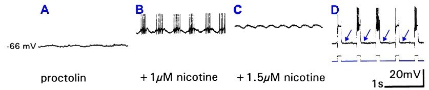
If nicotine excites motoneurons to fire action potentials, why do higher doses prevent action potentials?The answer to this question can be deduced from the figure below, in which an intracellular recording was made from a swimmeret motoneuron while nicotine was added in two doses, 1 µM and 1.5 µM. The ganglion was first treated with the peptide proctolin to induce rhythmic firing of action potentials in the motoneuron.
In panel A, proctolin induces a very shallow oscillation of the resting potential (-66 mV) that is not sufficient to reach the threshold for spikes. Addition of 1 µM nicotine (B) depolarizes the neuron (the resting potential moves upward) and enhances the oscillations, producing bursts of spikes. Increasing the dose of nicotine to 1.5 µM (C) further depolarizes the neuron, but spikes are no longer generated. Why not? In panel D, pulses of intracellular hyperpolarizing current (bottom trace) repeatedly force the membrane potential to a more negative value (arrows) for about a third of a second. When the neuron returns to its depolarized state between the intervals at its normal resting potential, it fires spikes. The most likely explanation is that the continuous severe depolarization leaves the neuron's sodium channels in their inactivated state, unable to open and fire spikes. Briefly returning the neuron to its resting potential allows the sodium channels to recover, so that they are ready to fire new spikes when they are again depolarized (panel D). Source: Braun, G and B Mulloney (1993) Cholinergic modulation of the swimmeret motor system in crayfish. J. Neurophysiology 70 (6): 2391-2398, fig 3. |
6. Summarize your data.
Prepare a PowerPoint file of no more than four slides to show the data you collected today. Include a title and your group's full names as part of the first slide. Each group's PowerPoint presentation will be distributed as a single page of four slides.
- On the first slide, include the labelled anatomical image
you selected in Part 2.
- From oscilloscope screenshots, present a few oscilloscope
traces that show the shapes of single extracellular action potentials.
Label clearly the horizontal timescale and the vertical voltage scale,
correcting for the amplification so that the vertical scale represents
voltage at the electrode.
- Include a screenshot of an excerpt from a LabChart record
that shows individual spikes in the spontaneous
activity you recorded. Label individual units
with numbers to mark axons that can be identified by their size.
- From your computer file of the response to nicotine, create an image of the full experiment to show the overall event, and also take screenshots of several enlarged sections (with an expanded timescale) to show details of firing patterns.
Email your finished PowerPoint summary to the instructors, preferably before you leave lab.
7. Clean up.
When you clean up, flush the suction electrode with water to prevent the saline from drying and clogging the tip. Also make sure you turn off the preamplifier. Rinse out your dissecting dish, and clean and dry your dissecting tools. Move any stray files from your computer's desktop into a folder for today's experiment, and place that folder in the main folder for your lab day.
Links
Supplement: Anatomy of the Crayfish Nervous System.
Appendix: Capturing Oscilloscope Screenshots
Appendix: Using EasyGraf Chart Recorders.
Appendix: Capturing Data with PowerLab and Chart.
© 2003, 2008, 2011, 2019 by Richard F. Olivo. Permission is granted to non-profit educational institutions to reproduce or adapt this Web page for internal use provided that the original source and copyright are acknowledged.