
Biological Sciences 300, Smith College | Neurophysiology
Lab 5: Computer Simulations of Membrane Potentials
http://www.science.smith.edu/departments/NeuroSci/courses/bio330/labs/L5sims.html
Revised: February 25, 2015
Bio 300 Home | Schedule | Laboratories | Administrative Information

MetaNeuron
This week, we will run computer simulations of membrane potentials using MetaNeuron, an application written at the University of Minnesota by Professor Eric Newman and Mark Newman. MetaNeuron is already installed on our laboratory computers (look for its icon in the dock), and you should launch it when you are ready to begin. Keep both this window and the MetaNeuron window open on your screen.
MetaNeuron is also available as a free download if you wish to have a copy for your personal computer.
Help files and interface controls:
MetaNeuron has two help files that are available from its menubar. For convenience, they are also reproduced (by permission) here: Lesson Descriptions provides details about the six separate simulations ("lessons"). Operating Instructions explains the versatile controls built into the program.
Those controls are also demonstrated in a video that you should watch now. Note also that when you drag a variable to change its value, as shown in the video, the numbers ordinarily change by 1, but if you:
- hold down the shift key, they change by 10
- hold down the command key, they change by 0.1
The plan for today:
We will explore five of the six simulations, in some cases doing quick explorations or demonstrations of the phenomena, and in others making a detailed study, including taking numerical data to plot. In some cases, you will be asked to make a screen shot of the relevant part of MetaNeuron's window. The next section explains how to do this. After your group has explored the five simulations, you will be asked to choose one simulation to work with more extensively, planning an experiment and acquiring data that you will summarize in a page to post and also demonstrate to the rest of the class.
|
A note on screen capture: MetaNeuron does not incorporate commands to print or save the plots that you generate, but you can accomplish this through the Mac's screen-capture routine. Pressing COMMAND-SHIFT-4 (together, briefly) changes the mouse cursor into a cross-hair cursor. Place this cursor in the upper left corner of any region that you wish to copy, and drag down to the opposite corner. You will see a rectangle that defines the region that will be copied. Release the mouse button, and you will hear a click. A "picture" has been taken of the region in the rectangle. It appears as a file on the desktop labeled "Screen shot" plus the date and time. Double-clicking a screen shot will open it in Preview. The images can also be dragged into Pages documents, resized, and later printed. Since it is easy to forget what each screen shot includes, it is good practice to change its name to something informative, and then drag the labeled screen shot into one (or more) new folders to which you give descriptive names. At the end of the afternoon, please drag your folders into the data folder for your lab day, to leave the desktop uncluttered for the next group. |
Reminder: Choose a simulation to work on from MetaNeuron's "Lesson" menu.
1. Resting potential (demonstration)
This simulation can duplicate the live experiment we did in Lab 3,
recording the resting potential while changing the concentration of K+ in
the outside saline. Demonstrate the same phenomenon by dynamically increasing
the Potassium "Concentration out" variable (click the cursor in the first box
and drag it to the right to increase the variable; you may wish to hold down
the shift key to increase it by steps of 10 mM).
Question to discuss with your partner(s):
why does the actual resting potential (yellow line)
become closer to the potassium equilibrium potential (blue line)
when the cell is more depolarized? (Hint: what happens to voltage-dependent
potassium channels if a cell is depolarized? Why would that cause the
resting potential to be closer to Ek?)
2. Membrane time constant (demonstration)
The next two simulations investigate passive membrane properties, responses that depend only on the physical characteristics of the axon membrane, without any active channels opening in response to depolarization.
This time constant simulation lets you inject a pulse of ions (the stimulus) while you view the change in membrane potential that occurs during a period of time. You have control over:
- the Membrane Resistance. A lower resistance allows charges to slip across the membrane more easily.
- the Stimulus Width and Amplitude (displayed in the red trace at the bottom) and its shape (square, or rounded like a post-synaptic potential).
- the Stimulus Train (how many pulses should there be, and how far apart in time?)
- the Graph duration: the default is 40 ms, but you can make it longer.
Restore the default conditions (File menu). Stretch the time axis (Graph) so the sweep duration is 150 ms (type in the new value). Now increase the stimulus width to 50 or 60 ms. Charges gradually accumulate until they are leaking out as fast as the stimulus is putting them in, and the potential reaches a steady state. Where have you seen this curve before? (Hint: in Lab 2.) Estimate the time constant of this simulated membrane. (Hint: clicking in the graph area brings up a cursor that you can move around, with its position in time and potential displayed at the bottom right. Reminder: the time constant is the time between the start of a capacitor's charging and the moment when it has reached 63% of its fully charged potential; we treated 63% as roughly two-thirds.)
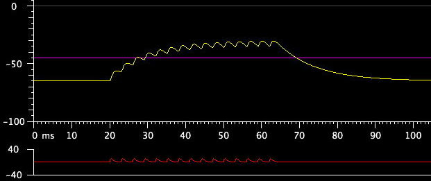
Observe a train of stimulus pulses: Restore the stimulus width to 1 ms, and in the Stimulus Train control box, set the Number to 10 or 15 while you increase the Period. Each short pulse puts in some charges; if the pulses are close together, the charges add up, while if they are far apart, the new charges mostly leak away without accumulating significantly. Change the stimulus shape to Synaptic Potential, and you will see what happens when an excitatory synapse is activated repeatedly to bring the postsynaptic potential above threshold for initiating a spike. This is called "temporal integration:"
3. Membrane length constant (demonstration)
The default display shows membrane potential vs. distance, with a stimulus
pulse introduced at the midpoint of this section of axon. Make the potential
easier to see by increasing the Stimulus Amplitude to 20 pA. The
display is similar to asking how far local circuit currents produced by
an action potential would spread, except that a square pulse instead of an action
potential creates the local circuit currents.
Examine the consequences of changing the Dendrite/Axon Properties.
First, estimate the length constant for the default conditions. Then make the
axon fatter by increasing its Diameter (press the command key to force
small steps). What happens to the spread of local circuit currents?
This is similar to the strategy of making giant axons to speed conduction.
Restore the diameter to 0.1 µm. Increase the Membrane Resistance,
one of the effects of wrapping myelin around an axon. (This simulation does
not let you explore the other consequence of myelination, lowering the membrane
capacitance.) What happens to the local circuit currents when the resistance
across the membrane is increased?
4. Axon action potential (detailed study)
The default settings show a stimulus pulse that eventually pushes the
membrane potential above threshold for making an action potential. Explore
the consequences of increasing and decreasing the Amplitude of
Stimulus 1. Why does
the action potential start sooner if the stimulus pulse is of greater
amplitude? To see a range of stimulus amplitudes, click its range box:
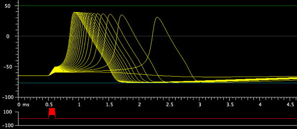
Decrease the Increment for the amplitude range to show more intermediate values, and then activate and rotate a 3D Graph of the display. Discuss what you are seeing with your partners.
Stimulus strength-duration curve. The effectiveness of a stimulus pulse in sending an axon above threshold depends on both the amplitude and width (duration) of the pulse. Conduct an experiment, recording your data to plot in a graph. Start with the default Width of Stimulus 1 (0.1 ms), and find the minimum Amplitude that is just above threshold for starting a spike. Write down the width and the amplitude for this stimulus pulse. Then double the width to 0.2 ms (use the command key to get small steps). Again find the amplitude that is just above threshold. Continue doubling the width and finding the minimum amplitude until the amplitude is no longer changing. Plot a graph of pulse width (x-axis) vs. amplitude (y-axis). Discuss why you can trade off stimulus width (pulse duration) and amplitude to reach threshold, and why there might be minimum values for each variable.
Low sodium experiment. After restoring default conditions, increase the Amplitude of Stimulus 1 to 150 µA, to make the stimulus more effective. Then do the equivalent of changing the outside concentration of Na+ by dynamically changing the Na+ equilibrium potential in the Membrane Parameters box (top left). What does this tell you about the cause of the action potential's peak?
Twin pulse experiment to explore refractory period. Restore default settings, and then make the following changes:
- Set the Sweep duration to 10 ms.
- Set the Amplitude of Stimulus 1 to 450 µA, so the action potential starts immediately after the stimulus pulse.
- Turn on Stimulus 2 and also set its Amplitude to 450 µA.
Examining conductances for Na+ and K+. With the twin-pulse range
still displayed, find the Conductances and Currents box and check "Show
ionic conductances." The conductance curves for Na+ (green) and K+ (blue) channels
will appear. Which one changes as the delay to the second pulse diminishes?
Why does it do so? Is the other conductance unchanged?
Restore default conditions, display ionic conductances again,
and examine the conductances as the Amplitude of Stimulus 1 is
varied from below threshold to far above threshold. Which conductance changes
most noticeably as the stimulus amplitude is increased and the spike starts
earlier?
Increasing and decreasing the density of channels. Restore default conditions and again show ionic conductances. In the Membrane Parameters box, change the density of sodium channels by dynamically altering the gNa max variable. This variable expresses the maximum sodium conductance, which depends on the number of channels packed into a unit area of membrane. Can you explain why the timing of the spike changes even though the stimulus amplitude is not being changed? Does the display of sodium conductance help you understand what is happening?
5. Axon voltage clamp (detailed study)
The default display shows the result of voltage clamping an axon at -5 mV for four milliseconds. The clamp depolarization is enough to open most of the axon's Na+ and K+ channels. The clamp voltage is set by the Amplitude of Stimulus 1, and the clamp duration is set by the Width. Choosing a range of Amplitudes will produce a family of voltage clamp currents (try this).
At this point, you should know enough about the MetaNeuron simulation to explore voltage clamping on your own. After you have a sense of how to manipulate the voltage clamp simulation, you are ready to move on to the next section of today's lab, a mini-project.
6. Simulation mini-project
With your lab partner(s), select one aspect of either action potentials or axon voltage clamping to explore further. Try to choose something that the simulation is particularly good at showing, such as the conductances or the ionic currents that result from an "experiment." It is a good idea to discuss your group's plan with the instructor before you dive into it. Then, when you are ready, launch the appropriate simulation and carry out your experiment. A copy of the MetaNeuron manual is on the desktop if you need to learn more about the program's functions.
Capture screen pictures, and compile a one-page "poster" of your mini-project using the Pages application that you launch from the dock. Your poster should state what the question was, show captioned examples of your experimental records, and have a conclusion that says what you found. Put your full names on the poster, and clip it to the blackboard. When everyone is ready, we'll have brief presentations of each group's project, and possibly some dynamic demonstrations at your computer. At the end of lab, tack your one-page poster to the bulletin board. Remember to gather the files and folders you created today and drag them to the data folder for your lab day, leaving the screen uncluttered for the next lab.
© 2015 by Richard F. Olivo. Permission is granted to non-profit educational institutions to reproduce or adapt this Web page for internal use provided that the original source and copyright are acknowledged.