
Biological Sciences 300/301, Smith College | Neurophysiology
Lab 2: Circuits and Amplifiers
http://www.science.smith.edu/departments/NeuroSci/courses/bio330/labs/L2ckts.html
Bio 300/301 Home | Schedule | Videos | Laboratories | Administrative Information
Our goal today is to work with simple electrical circuits to develop insights into electrical potentials (voltages) and currents. Throughout, there will be examples of how the concepts are applied in neurophysiology. We will also learn about the preamplifiers that we will use for future experiments. For today, we won't use the patch panel, but instead we'll connect cables directly to the oscilloscope.
1. Ohm's Law
We'll begin by observing Ohm's Law in circuits involving several resistors. Ohm's law says that when a voltage (an electrical "push") is applied to a circuit, the amount of current that actually flows through the circuit is inversely proportional to the total resistance the circuit offers. More resistance means less current:
E = I x R
volts = amps x ohms
Another law says that in a circuit, current can't pile up or disappear. The current flowing through every point in series in a circuit is the same. Consider this circuit:


The same current, I, flows through both resistors. Resistors in series add up, so in our circuit, the total resistance is 15,000 ohms. The voltage is 1.5 volts. By Ohm's Law, the current is
1.5 volts = I x 15,000 ohms
I = 1.5 / 15,000 = 10-4 amp = 0.1 milliamp
The total voltage of 1.5 volts is "used up" in pushing current through the two resistors. Most of the voltage is used pushing charges through the larger resistor. The voltage across either resistor can be calculated using Ohm's Law:

That is, 1.4 volts is used in forcing current across the big resistor, and only 0.1 volts is used across the small resistor.
Experiment: Measure the voltage across resistors in series for yourself. We have soldered two resistors together: 1000 ohms and 10,000 ohms (use the color code below to identify them). Set up this circuit with a 6-V battery and clip leads:

A word about polarity:
An isolated circuit of a battery and resistors does not have any point defined as zero (ground). When you attach a clip lead connected to ground, that point becomes defined as zero volts. Other locations in the circuit then take their relative positions with respect to zero. For example, if you ground the negative pole of the battery, that pole becomes zero and the other pole becomes +6 volts. If you ground the positive pole instead, the other pole becomes -6 volts. The oscilloscope trace will step up in the first case and down in the second, but the step will be 6 volts big in either case.
|
|
Use your oscilloscope to measure the voltage across each element of the circuit:
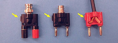
Attach a BNC/double-banana cable to channel one. [To get a very long cable, we will use our red BNC-BNC cable with a BNC/double-banana adapter on one end. Note the position of the ground tab on the double banana plug. The ground tab marks the side connected to the outside of the BNC plug or the copper braiding of the coaxial cable. These connect to the oscilloscope's electrical ground.]
Place a clip lead on each "banana" of the double-banana plug, and then attach the free ends of the clip leads on either side of various components. Measure the voltage and calculate the current for each component. Is the current the same in each part of the circuit? |

TIP: Although you are starting with the vertical scale set to 2 V/div, you should change it as needed so the difference between the zero baseline and the actual trace is large enough to see clearly. Similarly, you may benefit by placing the vertical position of Channel 1's baseline near the top or bottom of the screen.
|
measure voltage: |
volts (measured) |
current (calculated) |
|
across both resistors together |
|
|
|
across the small resistor |
|
|
|
across the large resistor |
|
|
Disconnect the battery when you are through.
Application: The principle that a voltage divides across resistors in series is important when recording with microelectrodes. These have very high resistances of 10 megohms (107 ohms) or more due to their very small tips. The microelectrode's resistance is in series with the input resistance of the amplifier, and the potential in the cell divides across the two resistances. Here's the circuit:

The amplifier can only detect the potential that appears across its input resistance. Any potential drop across the electrode is "lost." For example, if a cell's resting potential is -100 mV and the electrode and amplifier have equal resistances, the potential would divide equally across the two resistances. The cell would appear to have a resting potential of only -50 mV. To prevent this distortion, the amplifier's input resistance must be huge compared to the electrode's resistance. Amplifiers used with microelectrodes typically have an input resistance of 1012 ohms.
Problem: Estimate the proportion of the "real" potential that will be lost across a 10-megohm electrode if the amplifier's resistance is 1012 ohms. Would you consider the measurement error negligible?

2. Resistors and capacitors together.
A capacitor is a device that stores electric charge. Cell membranes are capacitors, and electronic circuits often have capacitors made of two thin sheets of metal foil with an insulating sheet between them, rolled up into a small cylinder. The amount of charge stored in a capacitor is proportional to its capacitance, C. The units of capacitance are "farads," but typical capacitors are in the microfarad range, and capacitances are routinely given in µF (10-6 F).
If a capacitor is connected to a battery as in the circuit at the left, electric charge will flow out of the battery as fast as it can until the capacitor is storing all the charge that it can hold. At this time, the flow of charge will cease, and the voltage across the capacitor will equal the voltage of the battery. The capacitor will continue to hold the charge indefinitely, even if the battery is disconnected.

Inserting a resistor in the circuit changes only one aspect. The rate at which charge flows out of the battery will now be limited by the resistor. Instead of charging up instantaneously, the capacitor will require some time to obtain all the charge that it can hold. During this charging time, the voltage across the capacitor will increase, starting at zero when the circuit is first connected, and reaching the voltage of the battery when the capacitor is fully charged.
Time constant: The time the capacitor requires to reach full charge depends on both the size of the resistance (big R means slow flow of charge, which means it takes a long time for the full charge to accumulate), and the size of the capacitor (a large capacitor holds more charge, so it takes longer to accumulate all the charge it can hold). The charging rate is exponential, and the time required to reach 63% (= 1 -1/e) of the full voltage applied is defined as the time constant of the circuit. The time constant (in seconds) is equal to the resistance (in ohms) times the capacitance (in farads). The time to discharge 63% is also equal to the time constant.
Time constant
TR=RRRxRC
(sec) (ohms) (farads)

Experiment: Observe the charging of a very large capacitor. We will use electrolytic capacitors, which require that one terminal (marked with a red dot or a +) be connected to the positive side of the circuit. Always be careful to observe this polarity. Clip together the following circuit except for the battery, which you should not connect until you are ready to observe the voltage across the capacitor. Use the single 1,000 ohm resistor, in the milk bottle.

- Set the oscilloscope's Horizontal Scale to 1 sec/div. Reset the horizontal trigger point to the left edge of the screen, using the Horizontal Position knob.
TIP: Always reset the horizontal position of the trigger point when you change the horizontal scale.
- Set the Vertical Scale at 1 V/div, and move the vertical position of the zero-volts baseline to near the bottom of the screen.
- Briefly connect a wire between the capacitor's two terminals to guarantee that the capacitor is fully discharged. Then connect in the battery and watch the voltage across the capacitor slowly increase as charges pile up on its plates. When the capacitor is fully charged, disconnect the battery. The charge on the capacitor remains, and the voltage across it will stay the same.
- Discharge the capacitor while observing the voltage by connecting together the two wires that formerly went to the battery:

Discharging is the inverse situation from charging. The capacitor slowly loses charge at a rate limited by the resistor till the voltage across the capacitor reaches zero.
Measure the time constant of the resistor-capacitor circuit:
- Charge the capacitor.
- Freeze the trace (by pressing the Run/Stop button) when the capacitor is almost fully charged. The trace will step up 6 divisions from the zero baseline when the capacitor is fully charged. Simplify your estimate by treating 63% as approximately two-thirds (66%), or four vertical divisions up from zero.
- Position the trace horizontally and vertically so that charging begins at the intersection of two major graticule lines. Count up four vertical divisions from zero, and measure the time (horizontal divisions) between the start of charging and the moment when the trace crosses the two-thirds line.
- If you wish, you may use the oscilloscope's cursors to help make these measurements. REMIND ME HOW
Calculate the capacitor's capacitance using the formula for the time constant. Substitute the values of the resistor you used and the time to two-thirds charge that you measured. Does your calculation agree with the value printed on the capacitor (within the precision of our rough methods)?
- Replace the resistor with one of approximately twice the resistance (2200 ohms), and charge the capacitor again. It should now reach full charge more slowly as the larger resistor further limits the flow of charge in the circuit.
Measure the time constant for this resistor, and again calculate the capacitance. Does the calculation agree with your previous one?
The capacitor-resistor circuit will be used again in the next section.
Application: When a voltage pulse is introduced in a nerve cell (either naturally, at a synapse, or experimentally, through an electrode), the shape of the voltage pulse gets lower and "rounder" as one records at greater and greater distances from the pulse's starting point. What one is seeing is the charging of a capacitor: in this case, the capacitor formed by the lipid bilayer of the membrane sandwiched between conducting solutions on each side. A famous model of an axon's resistance and capacitance is shown below. The axon membrane is represented as a series of resistors and capacitors, and the solution on each side as a series of resistors. The circuit is basically similar to the one you just put together.

Measuring current in a resistor-capacitor circuit. Suppose in the previous circuit we had measured the current flowing across the resistor instead of the voltage across the capacitor. We would have seen a large current flowing initially, when the capacitor was empty, and very little current flowing later, as the capacitor became more fully charged. When the capacitor reached full charge, the current flow would become zero.
We can qualitatively measure the current flow in a circuit by measuring the voltage across a resistor. (The actual value of the current can be calculated if we know the value of the resistor.) Ohm's law states that the voltage across a resistor is equal to the current times the resistance. A large measured voltage means a large current, and a small voltage means a small current.
Experiment:
- Adapt the circuit in the previous experiment to measure current by connecting the oscilloscope across the resistor rather than across the capacitor. Use the same resistors and big capacitor as before.

- Set the Vertical Scale to 2 V/div.
- Place the Channel 1 baseline in the vertical center of the screen by pressing the vertical posiition knob..
When you connect the battery, you will see its full voltage across the resistor, as only the resistor limits the flow of current. As the capacitor continues to charge, the charges accumulating on its plates tend to repel the new charges arriving. Current in the circuit flows ever more slowly, and as less current flows, the voltage across the resistor (I x R) becomes smaller and smaller. Eventually, when the capacitor is fully charged, no current flows, and the voltage across the resistor becomes zero (0 x R = 0).
When the capacitor is discharged through the resistor, the same situation occurs in reverse. Currents that flowed in a particular direction when charges were travelling to the capacitor now flow in the opposite direction as charges move away from the capacitor. During discharge, the voltage transient representing current flow across the resistor has the same shape but the opposite sign as it had during charging.
- Charge and discharge the capacitor circuit several times to observe this yourself. Do this first with the 1,000 ohm resistor, and then with the 2,200 ohm resistor

Application: One reason for understanding resistor-capacitor circuits is that many amplifiers are built with a "coupling" capacitor in series with the input resistance. The amplifiers are called "capacitor-coupled" or "AC" amplifiers. The DAM-50 amplifiers that we will use in future weeks can be either capacitor-coupled (AC) or direct-coupled (DC), depending on the setting of a front panel switch.
Our oscilloscopes also can be either AC or DC coupled, depending on the Coupling setting in the menu for Channels 1 and 2. The circuit diagram for the input to channel 1 on an oscilloscope is shown in the diagram below. The signal arrives at the BNC connector on the left, and it continues to the next part of channel 1's circuits on the right. In between is a three-position switch. It is represented as three open circles, one above the other, with an arrow from another circle just to the right. You are meant to understand that the arrow can point to any one of the three open circles, depending on whether the switch setting is AC, GND, or DC. (On our oscilloscopes, the switch is internal, controlled by the Coupling menu.)

In the diagram, the switch is set on AC. The path from the BNC connector to channel 1's amplifier goes through a capacitor (top position of the switch, as shown). If the arrow points to the bottom circle (DC setting), a wire bypasses the capacitor and the signal goes directly to the amplifier. In the middle setting (GND), the input signal just "hangs" there, not going anywhere, and the channel 1 amplifier is connected internally to ground.
AC and DC Coupling on an Oscilloscope
Experiments: Examine the difference between AC and DC coupling on your oscilloscope by looking at the same signal with both types of coupling simultaneously.
- Keep the connection you have to Channel 1.
- Set Channel 1's Coupling menu to AC coupling.
- Set Channel 1's vertical scale on 2 V/div. Set its vertical position at the middle of the screen.
Connect a second BNC/double-banana cable to Channel 2's input connector. Plug the cable's banana plugs into the banana plugs for Channel 1. [Be sure to align the ground tabs on the two stacked plugs, as in the photo below.] Channels 1 and 2 will receive the same signal.
- Turn on Channel 2.
- Set Channel 2's Coupling menu to DC coupling.
- Set Channel 2's vertical scale on 2 V/div. Set its vertical position at the bottom of the screen.
- Set the horizontal time scale to 100 ms/div.
- Arrange two clip leads to connect the banana plugs to the two terminals of the battery.

- Connect and disconnect one of the clip leads to the battery. Do this multiple times, trying to get a clean image on the screen. Observe the difference between Channel 1's and Channel 2's display of this same signal.
When the battery is connected, Channel 2's trace will step up 6 volts and stay there. When you disconnect the clip lead, Channel 2's trace will drop back to the baseline. Channel 2 is DC-coupled, and it shows steady potentials as well as the changes when you connect and disconnect.
Channel 1's trace, on the other hand, will step up 6 volts, but then rapidly return to the baseline even though the battery is still connected. The curve looks like the one you saw when you monitored the potential across a resistor when the big capacitor was charging. (The curve is faster because the oscilloscope's coupling capacitor is smaller.) When you disconnect the battery, Channel 1's trace transiently drops down 6 volts but then returns to the baseline. The curve is the inverse of what you saw when you connected the battery. Channel 1 is AC-coupled, and it shows only changes in potential, not steady potentials.

- Obtain a persuasive display (like this photo) by triggering on Channel 2, with the trigger point set one or two boxes in from the left edge. Select Normal Sweep in the Trigger Menu, not Auto, to keep the display from being overwritten immediately. Touch a clip lead to a battery terminal firmly but briefly to get a clean connection and disconnection.
Capacitor-Coupled Circuits Are Useful
Why would anyone ever build a capacitor-coupled circuit? We have just seen that capacitor-coupled (AC) circuits distort signals, eliminating steady voltages and showing only rapid changes. Why would anyone want a distorted signal? The answer is that an AC-coupled circuit is simpler to design because it is very stable (the baseline voltage never drifts away from zero), and in applications where steady voltages are not of interest, AC amplifiers and AC coupling in oscilloscopes are actually better. Action potentials recorded with extracellular electrodes are very brief, and AC circuits reproduce this transient voltage accurately. Since the baseline voltage is of no special interest for extracellular recording, nothing is lost by using an AC amplifier. (On the other hand, resting potentials and slow generator potentials do require direct-coupled DC circuits, since these signals contain steady or slowly changing components that would be filtered out by AC circuits.)
.
3. Preamplifiers for extracellular recording.
An action potential recorded extracellularly is a very small electrical change, typically tens or hundreds of microvolts. This would not be visible on our oscilloscopes even at their maximum vertical sensitivity. Consequently, a preamplifier is used between the electrodes and the oscilloscope. Typically, a preamplifier for extracellular recording has an amplification factor ("gain") of about 1000x.
Because the amplification factor is so large, any stray signals that are picked up by the electrodes or the wires (which act like antennas) are also amplified and can turn out to be quite substantial. The major sources of stray signals are the AC power lines and the room lights, both of which broadcast 60-cycle electrical interference. Neurophysiologists try to shield their experiments from electrical noise by using grounded baseplates, shielded cables (where a grounded wire braid intercepts the electrical noise), and differential preamplifiers.
Differential inputs. A differential preamplifier has two active inputs plus a ground (rather than just one active input and a ground, like most amplifiers). The amplifier inverts one of the two inputs and adds it to the other input. This is equivalent to subtracting one input signal from the other. Any noise component that is common to both signals is subtracted out, leaving the difference between the two signals for further amplification (hence the name "differential" amplifier). The amplifier's output is "single-ended," with one active wire and a ground.
In recording neural activity with a differential amplifier, one uses two electrodes and arranges the wires from them so that they are the same length and run next to each other. The two wires will pick up the same electrical noise, while the biological signals on them will be different. The amplifier's output shows the amplified biological signal with most of the electrical noise subtracted.
On the input block of our DAM 50 preamplifiers, the red input post is the non-inverting (A) input, the black post is the inverting (B) input, and the white post is ground. It is customary to connect the active electrode to the non-inverting input (red), and to connect the reference electrode to the inverting input (black). In this arrangement, when the preamplifier is connected to the oscilloscope, a positive voltage at the active electrode will produce a positive (upwards) signal on the oscilloscope screen.
Filtering the signal. Our amplifiers have electronic filters that can remove low- or high-frequency components of the signal being amplified.
Any electrical signal may be thought of as the sum of components of many different frequencies. For an action potential, the important components are around 1000 cycles per second (1 kHz). Riding along with this may be unwanted components such as low-frequency drift (below about 10 Hz), power-line noise (60 Hz), and high-frequency electron noise (above 10 kHz). By selecting appropriate filter settings, some or all of the unwanted frequencies can be filtered out.Low-frequency filter. As mentioned above, our preamplifiers have coupling capacitors on their inputs. These serve to block steady and slowly changing (low frequency) signals, allowing only quick transients to come through. We have already seen that if a capacitor is very large (like the big one we used in our test circuits), moderately slow transient signals will get through. If the capacitor is small (like the one that AC-couples our oscilloscopes), only very rapid transients get through. Different sized capacitors selected by the low-frequency filter (blue rectangle in the photo) create different degrees of filtering. The filter settings are identified by the frequency of the signal that is reduced to about half its actual amplitude. For example, a low-frequency setting of 10Hz means that signals of 10 Hz are reduced to half their real amplitude, signals below 10 Hz are reduced even more, and signals above 10 Hz are reduced less or not at all.

High-frequency filter. Our DAM 50 preamplifiers also have an adjustable high-frequency filter (red circle). High-frequency filter settings are named for the frequency that is reduced to half its real amplitude, with frequencies above the setting reduced even more or blocked completely. We will see the effects of high-frequency filter settings in a demonstration (below).
Filter Settings on DAM 50 Preamplifiers: The graph below shows the relative amplification plotted against the signal frequency for a DAM 50 preamplifier with its low-frequency and high-frequency filters at various settings.
The data were obtained by connecting a sine wave generator to the preamplifier's input. The sine wave amplitude was always 40 mV peak to peak. The amplifier's gain was set at 100, and the coupling mode was AC. The output signal was measured for a series of test sinewave frequencies between 5 Hz and 10 kHz (horizontal axis, a logarithmic scale). For each test frequency, either the low-frequency filter was set to each of its possible values (0.1, 1, 10 or 300 Hz) with the high-frequency filter at its most wide-open value (10 kHz), or the high-frequency filter was stepped through its possible values (100 Hz, 1 kHz, 3 kHz, 10 kHz) with the low-frequency filter at its most wide-open value (0.1 Hz). At each setting, the output signal was measured, and the amplification was calculated and plotted as a fraction of the maximum amplification.
The low-frequency filters reduce the amplification at the left (low) end of the frequency range. The high frequency filters reduce the right (high) end. The frequency range that remains for any combination of high- and low-filters is the middle zone between their two curves. For example, the arrow shows the span of frequencies that would remain with the low-frequency filter set at 10 Hz and the high-frequency filter set at 1 kHz.

In practice, both the high- and low-frequency filters are set by trial and error. The trick is to adjust the filters to block out distracting components of the signal (for example, low-frequency baseline drift and high-frequency electronic hiss) without reducing components of interest. Since action potentials have a major signal component at about 1 kHz, we have to be careful not to drop the high-frequency filter below its 1-kHz setting, or we will distort or even eliminate completely the action potentials that we are trying to see.
True story: Occasionally, a lab group thinks that they have not managed to get an experiment to work successfully, only to discover that they actually were getting excellent recordings, but were inadvertently filtering out the spikes.
Demonstration: Amplification and high-frequency filtering of your DAM 50 preamplifier.
The following section will be done as a demonstration by the instructor rather than as an exercise for each group. This video shows the demonstration.
|
Input signal: a square wave.
The oscilloscope provides a 3-volt square wave signal at 1 kHz frequency at a small tab near the bottom right corner of the instrument, as shown here. The 3V signal is far too big to feed directly into the preamplifier, which was designed to accept signals of a few microvolts or millivolts (3 volts is 3,000,000 microvolts!). To decrease this signal to a range that the amplifier can accept, we divide the 3V signal into two components by using the pair of 10k/1k resistors from the first experiment, as shown in the figure below. By sampling the potential across the small resistor (1,000 ohms), we acquire a signal that is less than 0.3 volts, small enough to feed into our amplifier. |
|

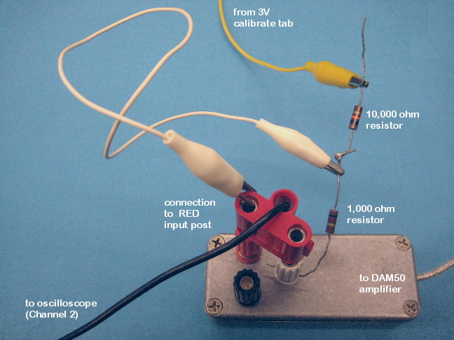
Dividing the 3V signal into two smaller signals by using large and small resistors. The white clip lead picks up the smaller voltage and connects it to the active input of the DAM 50 amplifier. The red double-banana plug samples that same signal and connects it to channel 1 of the oscilloscope.
Channel 1 will display the small square-wave signal that is connected to
the input of the DAM 50 amplifier.
Channel 2 will display the output of the
amplifier, after the signal has been amplified and
filtered.
The amplification is set on its lowest value (10x) by setting the DAM 50's Mode to DC and its Gain to 10x. We expect the output signal (on channel 2) to be ten times larger than the input signal (on channel 1).
Observing high-frequency filtering.Starting with the high-frequency filter set at 10 kHz, the least restrictive setting, we will reduce the high-frequency limit in steps (3 kHz, 1 kHz, 100 Hz) while observing the amplifier's output. We will see that filtering out the high frequencies distorts the output signal. The quick up-down portions of a square wave represent the highest-frequency components of that signal. When they are filtered out, the square wave starts to look rounded.
View a video of the demonstration
Question:What is the lowest high-filter setting that you could use for this 1 kHz signal without introducing unacceptable distortion?
[Demonstrating low-frequency filtering? For the curious, we can't test the effects of the DAM 50's low-frequency filter using this square-wave signal because we need DC coupling to get 10x gain, and the low-frequency filter is not in the circuit with DC coupling.]
Revised: February 7,
2015
Links
Appendix: Cables and Connectors.
Appendix: DAM 50 Preamplifier
© 2003, 2009, 2015 by Richard F. Olivo. Permission is granted to non-profit educational institutions to reproduce or adapt this Web page for internal use provided that the original source and copyright are acknowledged.