One of the major challenges in conducting a study of birds in migration is the fact that individuals are always coming and going. Unlike a breeding bird on territory, who can be predictably found on territory for weeks on end, a migrant may be at a stopover location for less than 24 hours. If a surveyor made only one count, at a time that no migrants happened to be on the move, they might conclude that the location was not a stopover location. If they happened to be there when a wave of migrants passed through, they might conclude that it was an excellent location. The way to address all the variability that comes with counting migrants is to have a large pool of sample locations, that are ssurveyed over a longer period of time. This approach helps to gain a bigger picture of the overall migration patterns, and prevents a single sample from having too great an influence on the conclusions. A three-year study was established to both increase sample sizes and avoid any potential bias due to year to year variability in seasonal weather and migration patterns.

The second challenge was having the sample locations geographically distributed within the Connecticut River Valley, so that no one location defined the migration pattern for the entire watershed. This is no small matter when the goal is to understand migration patterns and stopover geography in a 7.2 million acre (2.9 million ha)watershed ecosystem.

A guiding principle in developing the sampling scheme was to continue to rely on naturally occurring boundaries, in the same way the SOCNFWR was defined. The Connecticut River watershed is comprised of many sub-watersheds that range up and down the river's 420 mile length, making them naturally occurring sampling areas (Table 1). To insure that significantly large land areas were surveyed, only sub-watersheds 400 square miles or larger were considered.

Table 1: Major Connecticut River Tributaries

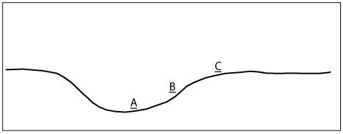
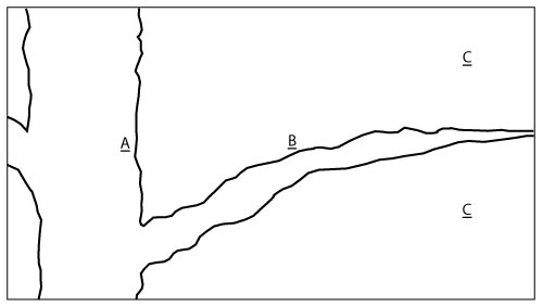
Since the goal was to understand the landscape ecology of how migrants were selecting stopover locations within the Connecticut River Valley, we designed a sampling scheme that would allow us to compare how migrants were using different areas of the landscape within the sub-watershed. Three geographic location types were defined for sampling within each sub-watershed (Figures 1 and 2).

Figure 1: Profile of sample locations

Figure 2: Aerial view of sample locations

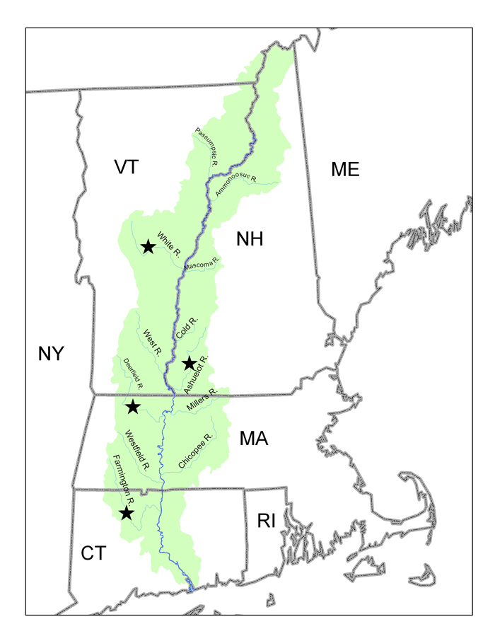
A sites were locations adjacent to the shore of the Connecticut River's main trunk.

B sites were positioned along the sub-watershed's major tributary that flowed into the Connecticut River.

C sites were upland locations, toward the sub-watershed's rim, that were unassociated with either the tributary or the Connecticut River.

In selecting the sub-watersheds, the two additional factors of habitat type and habitat structure had to be considered. Because the goal was to understand the influence of geography in the selection of stopover locations, we did not want the mixing of habitat types and different vegetation structures to confuse the geographic comparisons of A, B, and C sites. How a migrant might use a grassy field, compared to a forest, may vary considerably regardless of where the field or forest is located. This is a good question, but not the one we were asking. In the lower Connecticut River Valley the river is tidal, and has a greater percentage of tidal habitats, such as salt marsh or tidal flat when contrasted to the upper parts of the river. In the northern reaches of the river, conifers (evergreens) start to dominate tree vegetation. So as not to compare "apples and oranges," it was important to avoid comparing different habitat types, when trying to understand a migrant's preference was choosing one geographic location over another. All other factors being held equal, we wanted to assess the attraction or avoidance of river margins vs. uplands on a landscape scale. To insure we were comparing "apples to apples," sub-watersheds were selected that only fell in the long stretch of Northern Hardwoods/Mixed Deciduous forest habitat type that dominates much of the Connecticut River Valley. The sample watersheds selected were the Farmington River watershed in Connecticut, Deerfield River watershed in Massachusetts, Ashuelot River watershed in New Hampshire, and White River watershed in Vermont (Figure 3).

Figure 3: Subwatershed sample locations

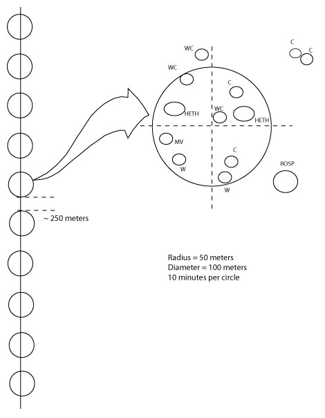
Actual migrant bird surveying routes, or transects, were then established in each of the selected sub-watersheds. Before laying out transects and conducting surveys, landowner permission was obtained. In selecting specific transect locations, all non-conforming forest habitats (e.g. wetlands, marshes, agricultural lands, built structures, scrub lands) were avoided to reduce sampling bias. Transects were also placed to avoid fragmented forest by following narrow trails that did not break the canopy, or through intact forests with the aid of topographic maps and compasses.

A survey transect was approximately 1.9 kilometers (1.2 miles) long, but in specific circumstances may have varied from the standard due to local conditions. Along the transect's length 10 point count circles were established, with each circle having a 100 meter diameter. The 10 point count circles were distributed evenly along the length of the transect (Figure 4).

Figure 4: Sample transect and point count circle

The point count circle's center was located along the transect by temporary flagging and a tree tag, so that each circle could be identified by a surveyor from week to week, or year to year. A point count circle was defined as 100 meters in diameter, centered on the transect pin or flag. To survey migrants, the volunteer surveyor would start walking at sunrise (approximately 6:00-6:30AM) along the transect and stop at each circle center marker. They would stay at that point to sample birds for 10 minutes, counting all the birds they saw or identified by sound. For the 10 minute count period, three categories of bird sighting locations were recorded on a standardized data sheet: 1)all birds seen or heard within the 100 meter diameter circle, 2) all birds outside the circle, and 3) birds flying over the circle. The end of the transect at which the surveyor would begin counting alternated between weeks. This avoided the bias of the transect being surveyed in the same direction, at the same time of morning, every week. To reduce surveyor variability, annual training workshops were held prior to the start of each season for all volunteer surveyors, who had been previously identified as intermediate to accomplished birders.

Within each of the four sub-watersheds, 12 survey transects were established: 3 A site transects, 3 B site transects, and 6 C site transects. The 6 C sites allowed a pooling of the river/tributary locations (A, B, totaling 6) that would permit an equal comparison with the 6 dry upland sites.

During the spring migration period, 5 surveys were conducted (Table 2). Also, 1 additional survey was conducted during the breeding season (later in June) so that a preliminary comparison could be made between the number of birds counted during migration and the breeding season. While these Saturdays were the target dates, some count days were deferred to the following Sunday or Monday due to weather or scheduling issues. The dates from late April through early June were selected to cover the spring migration window of Neotropical migrants in the SOCNFWR. (Although some bird species migrate earlier, they are generally not Neotropical migrants). The final survey was scheduled to end before any but the earliest birds of the year fledged. As a result, surveys were conducted on 6 spring dates, each year, for 3 years.

On each survey date, 12 transects were surveyed simultaneously in each of the four sub-watersheds, for a total of 48 surveys on each date. For each year of the study, surveys were simultaneously conducted by trained observers on the same six dates, all using the same methods. This resulted in a four sub-watershed total of 288 transect surveys per year, or a total of 2880 point counts per year.