
Biological Sciences 330, Smith College
| Research in Cellular Neurophysiology
Using the Digital Storage Oscilloscope
Revised: February 18, 2019
In our first laboratory, we will review the features of our digital storage oscilloscopes. When you arrive, you and your lab partner(s) should sit near one of the equipment racks. Please leave your coat and backpack in the coatrack near the door.
We will use oscilloscopes for viewing action potentials picked up by extracellular electrodes, but today we will look at pre-recorded demonstration signals instead. Our tasks today will be:
- to tour the oscilloscope to learn the function of each major group of controls.
- to look at demonstration signals and manipulate the way the signals are displayed.
The description of the oscilloscope's controls opens in a separate window so that you can easily refer to it later. Read about the history of oscilloscopes (below) and the different control sections (in the supplement) before you come to lab, so you will have an overview of the different functional groups before we use them.
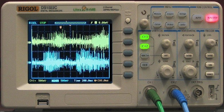
Rigol DS1022C Digital Oscilloscope
A Brief History of Oscilloscopes
An oscilloscope is an instrument for displaying electrical potential (the vertical scale) against time (horizontal scale). The first oscilloscopes were analog instruments. They were built around a "cathode ray tube" (similar to the picture tube in an old TV), which focused a beam of electrons to create a bright spot on the face of the viewing screen. Circuitry inside the oscilloscope swept the spot horizontally across the screen at a steady rate to establish the time axis. A knob on the control panel allowed the experimenter to select a particular horizontal sweep speed from a series of choices that were calibrated in seconds (or milliseconds) per horizontal division.
The electron beam could also be moved up and down on the screen by circuitry that amplified the voltage signal that was fed into the oscilloscope. An example of a signal is a series of amplified action potentials from a nerve. Again, a knob on the control panel selected the sensitivity of the vertical axis, in volts or millivolts per vertical division. The experimenter adjusted the vertical sensitivity so that the signals of interest filled the screen but did not overflow it.
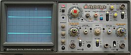
For many years, this lab course used "hybrid" analog/digital oscilloscopes that were analog oscilloscopes with an important additional feature: they could take digital samples of the signal, save them in memory, and replay them repeatedly to the screen, thereby "freezing" the trace on the screen. (They could also show traces one after the other without freezing them, in ordinary analog mode.) This hybrid technology was one early way of creating digital storage. Like many other analog or digital oscilloscopes, our instruments could also display two traces, for observing two voltage signals simultaneously.
You can see a larger version of this image, and you can also read an older version of these lab instructions, describing how to use the Hitachi oscilloscopes.Notice that there are a large number of knobs and switches on the control panel, which students mastered during the semester.
Analog oscilloscopes and hybrid analog/digital oscilloscopes are still manufactured, but most digital storage oscilloscopes now are fully digital. They are essentially specialized computers with graphics screens that emulate analog oscilloscopes. Their digital circuitry takes many thousands of samples per second of the incoming voltage signals, stores them as numbers in the computer's memory, and plots them instantly on the screen. Knobs on the control panel select the horizontal scale (seconds/division) and vertical scale (volts/division) for the display, just as they did on the original analog oscilloscopes.
Our Rigol DS1022C digital storage oscilloscopes
have simplified control panels compared to analog
oscilloscopes because many functions are relegated to menus
on the screen instead of being controlled by switches on the
panel. In spite of their apparent simplicity, digital
oscilloscopes usually have many more features than their
analog predecessors did.
Prerecorded Signals to Display
To investigate the oscilloscope's functions, we need a real signal to look at. Your computer has two sets of prerecorded two-channel sound files that we can view with the oscilloscope:
1. Sound Waveforms (steady tone, fade-up, and frequency sweep)
After you have launched the pop-up window, press a "play" triangle to hear a sound (press the "pause" button to stop the sound). The same sound is recorded on both channels.
NOTE: more than one sound can play simultaneously, probably not something you intend to do. Stop a sound before starting a new one.
2. A recording of neural activity.
This sound repeats automatically once you press play in the pop-up window. The two channels have different signals that were recorded simultaneously.
The recording shows bursts of action potentials in nerves leading to swimmeret muscles from two adjacent abdominal ganglia in a crayfish. Each nerve has about 30 motoneuron axons in it. Electrodes pick up action potentials from these neurons, which look like vertical spikes at a slow timescale. Spikes from different neurons appear to have different amplitudes in extracellular recordings, which allows us in many cases to follow the firing of individual neurons (especially the biggest ones). The neural activity is rhythmic: the axons in this nerve are active for a short period, then quiet, then active again, alternately exciting the opposing muscles that move the swimmerets back and forth.
To connect your computer's sound output to the oscilloscope's input for observing the signal on the screen (this may already have been done):
- Plug a mini-stereo cable into the computer's headphone output on the back of the screen (marked with a symbol for headphones).
- plug the cable's other end into a stereo jack on the patch panel under the oscilloscope. The green and blue BNC cables should already connect the patch panel to the inputs for CH1 and CH2.
- Turn on the stereo speakers mounted below the
patch panel, and adjust the volume to a low level. You
should hear the sound from the recorded source that you
have selected. (If you tire of listening to the sound,
you can turn off the stereo speakers whenever you
wish.)
Activities To Do in Lab
Vertical, Horizontal and Trigger Settings
The Big Three:
Three knobs in the main control panel are for important settings that are adjusted frequently. To explore these settings, play the steady tone from the Sound Waveforms signals and activate channel 1 by pressing the CH1 button to the right of the screen (in the VERTICAL box). At this point, channel 1 should display the steady tone signal, a sinewave. We will explore:
- vertical sensitivity and position,
- horizontal sweep speed (time) and position, and
- trigger level.
Press the vertical POSITION knob to place the baseline (and therefore the trace) at the center of the screen. Adjust the vertical SCALE knob to make the signal fill most of the screen but not overflow it. The scale you choose will be displayed below the screen in units of volts (or millivolts) per vertical division (see the oscilloscope's controls supplement for a full description):
Adjust the horizontal scale
The horizontal scale may or may not be optimal for examing the signal. Try various settings to see what they show. Slow sweeps (100 ms per division or slower) will show you the signal as a smear of solid color. Fast sweeps (5 ms per division or faster) will show you the sinusoidal signal's shape. In practice, select whichever horizontal scale shows you the aspect of the signal that you are trying to see.
For now, select a horizontal scale that displays a few cycles of the sinusoidal wave (1 ms is a reasonable choice).
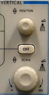
Menu for Channel 1 (vertical settings)
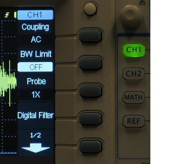
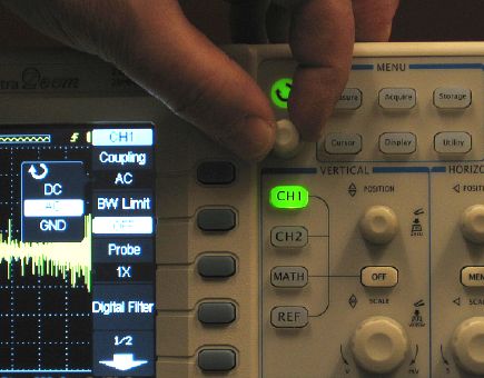
The knobs for the vertical channels are supplemented by a menu for each channel. To activate the menu for channel 1, press the green "CH1" button. A drop-down menu will appear at the right edge of the screen. Pressing the gray button next to the arrow at the bottom brings up a second menu for channel 1. Pressing the gray button at the top of this menu takes you back to the first one.
|
Menu 1 (of 2) for channel 1
|
Menu 2 (of 2) for channel 1
|
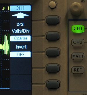
The menu for channel 2 is identical to channel 1. It is activated by pressing the green CH2 button.
Selecting the input coupling for a channel: AC or DC?
We will be interested mostly in the top item in the first menu, the input coupling for the channel. It has three settings:
- AC coupling, for displaying rapid changes in the signal but not slow or steady potentials. We will usually choose AC coupling for looking at action potentials recorded with extracellular electrodes.
- DC coupling, for looking at steady (or changing) voltages, such as resting potentials recorded with intracellular microelectrodes.
- Grounding the input circuits. This disconnects the signal coming in through the channel's BNC jack while internally connecting the channel's circuitry to ground (GND), a potential of zero volts. This is useful for establishing the vertical position of the trace on the screen.
To change the input coupling, press the uppermost gray button, next to the "Coupling" setting. A subsidiary menu will pop up. In this example, it shows that channel 1's input coupling is currently set to AC.
|
|
The circular arrow reminds you that adjustments are made with the menu adjust knob at the top, which lights up. Change the setting and then press the knob to enter your choice.
|
|
Here the input coupling has been changed to DC:
|
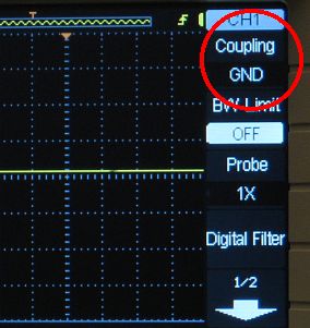
And here, to GND. Note that the trace is now flat because channel 1 has been internally connected to zero volts (ground). The signal on the input connector is left "hanging," not going anywhere.
|
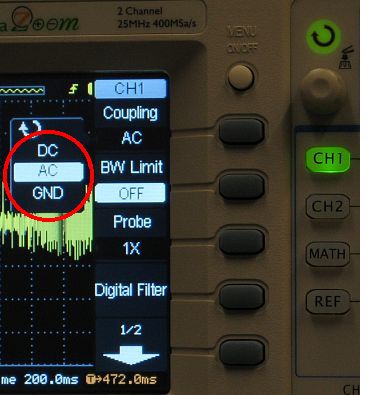
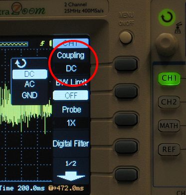
For today, set channel 1's input coupling to DC. Press the menu adjust knob to enter your choice.
Display Menu: Dots vs. Vectors
The display menu is launched by a button in the "Menu" area at the top left of the control panel. Several settings are important to us. In the first (of two) display menus, the top item is Type, which can be "Dots" or "Vectors." Pushing the gray button toggles between these two settings.
|
"Dots" shows each sample as a point...
|
while "Vectors" draws lines between the points.
|
We usually want "Vectors." The other items on the first display menu are:
- Clear to erase the screen.
- Persist to determine whether old traces remain on the screen (as dim lines), with the newest trace written on top as a bright line (Infinite), or instead whether the previous trace will vanish when the new one is written (Off).
- Intensity to adjust the brightness of the traces by turning the menu adjust knob. We usually want a very bright trace.
- The down arrow takes us to the second display menu.
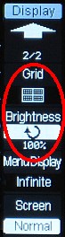
In the second display menu, we can
- choose from three different styles of grids (we want the one with the most boxes);
- adjust the brightness of the grid by pressing the gray button next to "Brightness" and turning the menu adjust knob.
- set whether menus will be displayed until we make them go away (Infinite) or instead fade away after a predetermined time (selected from a list);
- reverse the light/dark layout on the screen (bright screen, dark traces). A reversed screen can be helpful if we wish to save images of the screen for printing, but many people find a bright screen unpleasant to look at.
Triggering
To examine triggering, initially select the frequency sweep from the Sound Waveforms signals. (Remember to pause any other sound that is playing.)
The trigger controls determine the horizontal position on the screen of the digital samples as they are being taken and displayed. It allows the experimenter to line up a particular point in the signal (for example, the rising phase of an action potential) at the same place on the screen for trace after trace. Without triggering, the events would appear at random places on successive sweeps and be difficult to study.
To control triggering, you specify:
- the voltage level that the signal must pass through,
- the direction (slope) in which it is going (upwards, positive slope, or downwards, negative slope).
- the source for triggering, chosen from:
- channel 1
- channel 2
- an external trigger signal (connected to a BNC jack on the bottom right of the front panel)
- the 60-cycle AC power line.
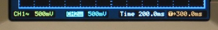
The trigger circuits examine the incoming waveform and line up the display based on when the trigger conditions are met. Trigger settings are displayed in yellow at the top right edge of the screen:
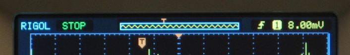
This example shows that triggering is set for a rising edge (positive slope, symbolized by the upwards arrow). The source is channel 1, indicated by the "1" inside a yellow box. The voltage level for triggering is (+) 8.00 mV, set by the trigger level knob. Pressing the knob forces the trigger level to zero volts, from which it can be adjusted up or down.
The example also shows the position of the trigger point in time. At the top, the zig-zag line represents the entire memory for the display, and the blue box represents the memory actually displayed on the screen (in this case, all of it). The orange "T" above the box shows where the trigger point occurs within the memory. The black T in a solid orange arrow also shows where the trigger moment occurs within the grid. The location of the trigger point is controlled by the horizontal position knob. Pressing that knob will force the trigger point to the horizontal center of the display.
![]() The
trigger moment is also displayed numerically at the bottom
right of the screen. Positive numbers indicate times
before (to the left of) the center midline, negative
numbers after the midline. In this example, the trigger
moment is 300 ms before the midline. Since each box is worth
200 ms, the trigger moment should be 1 1/2 boxes to the left
of the midline. You can see (from the image above) that is
indeed where it is.
The
trigger moment is also displayed numerically at the bottom
right of the screen. Positive numbers indicate times
before (to the left of) the center midline, negative
numbers after the midline. In this example, the trigger
moment is 300 ms before the midline. Since each box is worth
200 ms, the trigger moment should be 1 1/2 boxes to the left
of the midline. You can see (from the image above) that is
indeed where it is.
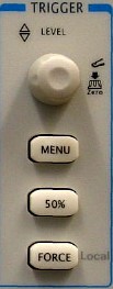
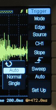
Trigger Menus
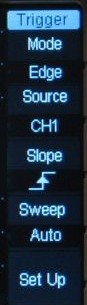
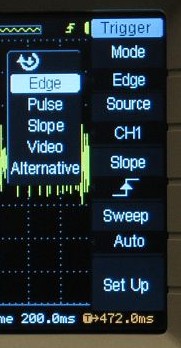
Many important trigger functions are controlled by the trigger menu, shown at the left. The trigger menu is probably the menu you will return to most often. There are five major trigger functions on the menu: mode, source, slope, sweep, and setup. Pressing an adjoining gray button brings up a submenu and lights up the menu adjust knob. Turning and pressing the knob selects a setting.
|
|
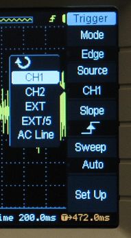
The trigger source will usually be CH1 or CH2. A channel can serve as a trigger source even if its display is turned off.
|
We will select the slope depending on the signal we are looking at, choosing positive (upwards) or negative (downwards)
|
|
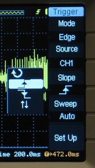
Sweep: Auto makes the trigger wait briefly for an appropriate signal, but then forces a sweep if no trigger occurs.
|
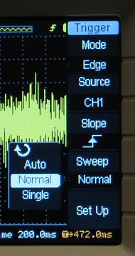
Sweep: Normal gives us full control. The display waits indefinitely until the signal meets the trigger conditions.
|
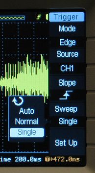
Sweep: Single is Normal sweep with an additional feature: the first captured trace is held until you press the Run/Stop button.
|
|
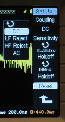
Trigger Set Up allows us to choose an absolute voltage level (DC coupling) or a relative change in voltage (AC).
|
Some general comments about triggering:
|
|
Triggering on a sinewave
Now it's time to work with triggering. Turn off the frequency sweep signal and turn on the steady tone.
While playing the signal, launch the trigger menu and select:
- edge mode
- channel 1 source
- positive slope
- normal sweep
- DC coupling from the set-up menu
(1) Press the horizontal position knob to place the trigger moment at the center of the screen. Slowly adjust the trigger level control while watching the screen. You should see the voltage crossing the center of the screen rise or fall as you change the trigger level. You are telling the trigger circuit to find out when the signal crosses a particular level, and to align the sweep so that the sample that meets that criterion is at the center of the screen.
If you change the level to a voltage higher or lower than this particular signal supplies, the display will not draw any new traces. (The last trace acquired will remain on the screen until the next successful trigger event.)
(2) Adjust the trigger level so it is about halfway between the peak and trough of the sinewave. (Pressing the trigger level knob will do this for you.) Examine the trigger slope by relaunching the trigger menu, pressing the gray button for slope, and switching the slope back and forth between positive and negative while watching the screen. (Remember that you must press the menu adjust knob to enter your choice.) The trigger level should not change, but the sinewave should pass through the trigger level in opposite directions, upwards or downwards, depending on the slope you have chosen.
(3) Investigate how to place the trigger moment horizontally on the screen wherever you like. Adjust the horizontal position control so the trigger moment shifts left or right from the center of the screen.
Cursors for Measurements
Continue to play the steady tone and establish a stable triggered sweep (successive sweeps will overlap each other). Expand the horizontal scale so that approximately two complete cycles of the sinewave fill the screen. Freeze the display by pressing the Stop button. Look at the value of a horizontal box (the time scale at the bottom of the screen), and estimate the time for one complete cycle of the sinewave. Similarly, look at the vertical scale and estimate the peak-to-peak voltage of the sinewave. This is the traditional way of making measurements from an oscilloscope screen.
Tip: Adjust the vertical and horizontal position controls to place a convenient point on the signal exactly on the corner of a graticule box, and then measure by counting in appropriate units from the horizontal and vertical graticule lines to the place where the signal repeats the convenient point that you selected.
 Since
the voltage of the signal is represented by numbers in the
oscilloscope's memory, it was easy to add a feature that
helps you measure time and amplitude. In the menu button
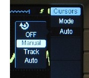
area at the top left is a button labelled "Cursor." Press
that button to bring up the cursor menu, press "Mode"
and select "Manual" cursor. A new menu will
appear.
Since
the voltage of the signal is represented by numbers in the
oscilloscope's memory, it was easy to add a feature that
helps you measure time and amplitude. In the menu button
area at the top left is a button labelled "Cursor." Press
that button to bring up the cursor menu, press "Mode"
and select "Manual" cursor. A new menu will
appear.
Select "X" for the Type of manual cursor. This will allow you to make measurements horizontally of the difference in time between two points. In the example below, the time between two extracellular action potentials is being measured. The Source was set to CH1, and then the button for Cursor A was pressed to activate the leftmost cursor. Cursor A was adjusted to the location shown. Then the Cursor A button was pressed again to turn it off, and the button for Cursor B was pressed (it remained the active cursor at the time the photo was taken -- its "adjust" label is highlighted). [Caution: you can have both cursors activated simultaneously, for shifting both of them together without changing the time between them. This is not usually something you want to do.] The delta-X measurement shows the time between cursors, 1.68 ms. This time is also shown as the equivalent frequency, 1/delta-X, which is 595.2 Hz.
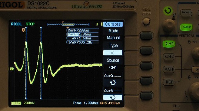
(4) Use manual cursors to measure the time between equivalent points on the steady sinewave you are displaying. What is the frequency of the sinewave?
To make vertical measurements of a difference in voltage, select "Y" for the Type of manual cursor. Cursor A and Cursor B are now horizontal lines instead of vertical ones. By activating and positioning each cursor in turn, the voltage difference between them is measured. (It is exactly 1.00 V for this highly amplified action potential.)
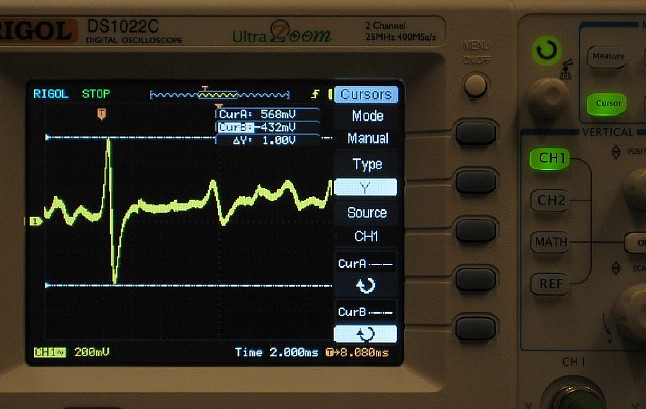
(5) Use manual cursors to measure the peak-to-peak amplitude of the sinewave you are displaying.
To turn the cursors off, press the Mode button again, and cycle from Manual to Off.
Trigger and make measurements from recorded neural activity
To develop your skills, you and your lab partners should now display, trigger on, and measure signals from neurons. Launch the window that plays a recording of neural activity.
The recording shows bursts of action potentials in nerves leading to swimmeret muscles from two adjacent abdominal ganglia in a crayfish. Each nerve has about 30 motoneuron axons in it. Electrodes pick up action potentials from these neurons, which look like vertical spikes at a slow timescale. Spikes from different neurons appear to have different amplitudes in extracellular recordings, which allows us in many cases to follow the firing of individual neurons (especially the biggest ones). The activity is rhythmic: the axons in this nerve are active for a short period, then quiet, then active again, driving the swimmeret appendages back and forth.
(6) Look at this activity initially at a slow timescale, to see the repeating bursts of action potentials. You will need to:
- display both channel 1 and channel 2
- select appropriate input coupling (AC is better) and vertical scales and positions that put both signals on the screen
- select a slow horizontal scale that lets you see more than one burst
- place the trigger point near the left edge of the screen
Freeze the traces (RUN/STOP button), and use horizontal cursors to measure the time interval between the start of successive bursts on the same channel. The blue trace (channel 2) will be easier to use because the bursts start very sharply.
(7) Then return to an active display by pressing the RUN button. Switch to a fast timescale (1 ms or 500 us) so you can see individual spikes. Place the trigger point in the middle of the screen by pressing the horizontal position knob. Trigger on single spikes on channel 1 by adjusting the trigger level.
Tip: Turn off channel 2 while you investigate spikes on channel 1. This will give you more screen area for channel 1, so you can stretch out the vertical scale. You will find it easiest to see the same spike over and over if you set the trigger level high enough to detect only the largest spikes.
When you are triggering successfully on a large spike, investigate:
- the effect of switching trigger Sweep between auto, normal, and single
- on single sweep, the action of the run/stop button
- on a trace that shows a good example of a big spike,
estimate the width of that spike by looking at how
many horizontal grid boxes it spans and noting the time value of
each box.
HINT: stretching out the timescale will make it easier to estimate the spike's width. - with a trace stopped, and cursors turned off, examine how you can shift the section of memory displayed on the screen by turning the horizontal position button. The blue box around the zig-zag line (at the top of the screen) shows where in memory the displayed samples reside. You will see that you can scroll forwards and backwards in memory to review much more activity than can fit on the screen at this fast timescale.
Acquire Menu: Normal
and
Peak Detect
Aliasing. There is one more fairly subtle setting to investigate today using pre-recorded neural activity. But first, let's meet the concept of "aliasing." When digital samples are taken at a relatively slow rate from a signal that is changing at a much faster rate, the samples can't represent the shape of the signal accurately. Instead, they create a series of points that occur at unrepresentative moments within the signal, creating an "alias." The usual example for this is a fast sinewave (red in the diagram below) sampled at a slow rate (the circles). Each sample catches the sinewave at a different point in its waveform. When the points are connected (blue curve), the apparent signal looks plausible, but it misrepresents the actual (red) signal (the blue sinewave is much slower).
Source: Wikipedia article on
"Aliasing"
We run into this problem if we display a train of spikes at a very slow timescale (eg, 500 ms/division). At such a slow sweep, samples are taken at a few unpredictable points within each action potential, and the display misrepresents the heights of the action potentials.
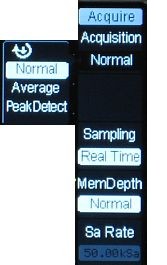
Luckily, our oscilloscopes provide a remedy for this in the Acquire menu (its button is in the Menu control area). The first item, Acquisition, allows us to choose between Normal, Average, or PeakDetect. We'll discuss Averaging in another lab, but the difference between Normal and PeakDetect is relevant here.
|
|
|
|
|
|
|
The only disadvantage of PeakDetect acquisition is that on fast sweeps (shown below), the trace looks "fat." |
|
|
|
|
 On
Normal acquisition, samples are taken at a
regular rate that depends on the horizontal
timescale. The image below shows three identical
repeats of the same burst of action potentials,
triggered on a very large spike. The horizontal
scale is slow, 200 ms. The three repeats don't look
very similar because the individual spikes are
being sampled at a rate too low to represent them
well.
On
Normal acquisition, samples are taken at a
regular rate that depends on the horizontal
timescale. The image below shows three identical
repeats of the same burst of action potentials,
triggered on a very large spike. The horizontal
scale is slow, 200 ms. The three repeats don't look
very similar because the individual spikes are
being sampled at a rate too low to represent them
well.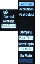 If
instead the same data are sampled with
PeakDetect acquisition, the circuitry takes
samples at a very high rate but saves only the most
positive and most negative values within the time
represented by each column of pixels on the screen.
When those high and low points are connected,
spikes are drawn with their full height and look
more uniform. The three repeats of the same data
now look identical.
If
instead the same data are sampled with
PeakDetect acquisition, the circuitry takes
samples at a very high rate but saves only the most
positive and most negative values within the time
represented by each column of pixels on the screen.
When those high and low points are connected,
spikes are drawn with their full height and look
more uniform. The three repeats of the same data
now look identical.
(8) Investigate the effects of switching between Normal and PeakDetect acquisition while displaying the neural data at a slow sweep, such as 200 ms/div.
Display Menu:
Persistence of the trace
Our final trick for today is to explore the Persistence setting in the Display menu. In the left figure below, a spike triggers a sweep with the Persistence set to Off. On the right, the same spike triggers several sweeps with the Persistence set to Infinite. The most recent sweep is the bright trace, with previous sweeps appearing as overlapping dimmed-out traces. We can see that the shape of the triggering spike is fairly uniform in each trace, but the activity that follows the spike is not the same from trace to trace.
|
|
|
(9) Explore the use of persisting traces, using pre-recorded neural activity displayed on a fast sweep, as in these examples.
As the weeks go by, you will become more intuitively familiar with these oscilloscopes. Refer back to this lab as necessary to review the features and controls. We'll add additional details when we need them as the semester goes on.
Links
Appendixes: Rigol Digital Oscilloscope
© 2008, 2011, 2013, 2016 by Richard F. Olivo. Permission is granted to non-profit educational institutions to reproduce or adapt this Web page for internal use provided that the original source and copyright are acknowledged.