Research Log
|
Jacob Last
Smith College
Summer 2005
Prof. Judy Franklin
|
|
|
Week One
Started on Tuesday. After doing some administrative stuff, we
started talking about possibilities for the project. It seems like
we'll be using Reinforcement Learning (RL) applied to real time
processing of musical audio signals, rather than MIDI data. We haven't
yet decided what exactly the application will be, although we talked
about a few possibilities:
- RL component will learn to apply various audio filters to a
player's live playing; reward could come from yes/no feedback from the
player or from some other judge.
- RL component could learn a mapping from live MIDI control stream
(from the iCube system, for example) to audio filters. Again
feedback might come from the player somehow.
- ...
We've decided to use Pd (Pure Data) and/or Max/MSP, two similar real
time object-based audio and midi programming environments, to
implement our system. One can write externals for these systems
in C in order to implement algorithms that would be too slow,
impossible or very messy to program in the graphical environment. Pd
and Max/MSP have very similar frameworks for developing externals, due
to their common origin in the work of Miller Puckette. Pd has the
advantage of being open source (and therefore free), but lacks the
polish and documentation of Max/MSP (a commercial product).
My week's goal was to write a simple external for one of the
systems. First I was intending to write a Max external, but I found
out quickly that the version of Max installed on my OS X system is
4.2.1, which only supports externals compiled in the CFM binary
format, which is a holdover from Mac OS 9 and earlier, and which
neither gcc or xcode can produce. The latest version of
Max/MSP (4.5) supports the newer Mach-O binary executable
format. We are in the process of obtaining Max/MSP 4.5, but in the
meantime I've decided to pursue Pd, since it supports
Mach-O-style externals, as well as using flext...
There exists a very nicely written and documented C++ wrapper layer
called flext, which allows
one to write externals once for flext, then compile them specifically
for Pd or Max/MSP on any platform: Linux, Mac OS X, or Windows. I've
decided to learn to write externals with flext rather than
writing directly for the Pd or Max API for a couple reasons: (1) it is
obviously nice to have the platform independence, (2) it actually
seems cleaner and easier than either of the native APIs, and (3) if we
later decide to use Max/MSP rather than Pd (once we have the 4.5
version), it will be relatively painless to switch. Here are some of
my notes on installing and compiling Pd and the flext libraries on OS
X
There are several binary distributions of Pd available for OS X, which
at first I was wary of, because I knew I'd need the source tree, and
wasn't comfortable with the idea of having a big old Pd.app in
/Applications/. Fortunately this works out fine as I'll show.
(There are some Pd installers for OS X that have been made which include a
collection of externals libraries, but I chose to use the one available
straight from Miller Puckette's website (linked above) in order to keep it
simple.) The install couldn't be easier; just drop Pd.app into the
applications folder and you're ready to go. I wanted a UNIX-style install
of Pd in order to install the flext library and headers though, which I actually
accomplished simply by symlinking:
ln -s /Applications/Pd.app/Contents/Resources/ /usr/local/pd
I am really starting to like OS X! Anyway, now on to installing flext.
Downloaded the flext source distribution from the flext link above,
untar'ed into /usr/src. Then I just modified the config file and pointed
it at /usr/local/pd, etc. and the compile went fine. I chose
/usr/local/pd/flext to install the flext library to.
I downloaded the flext-intro.pdf document as well as the archive to
tutorial examples from the flext web site. For some reason the signal
based externals won't compile, which is something we might eventually need
to contend with. The non-signal based externals all compiled fine, and once
installed in the /usr/local/pd/extra directory, the example
patches from the tutorial distribution run fine.
I found the answer to the signal externals not compiling...need to add -framework veclib to the linker flags for OSX 10.3...found this on the PD mailing list archives (http://lists.puredata.info/pipermail/pd-list/2004-01/016979.html)
I wrote a simple external of my own from scratch called
accum. It has two inlets and two outlets. Inlet 0 receieves
floats and adds them to a running sum. Inlet 1 sets the variable
maxiumum. When the running total exceeds maximum, the object
sends a bang to Outlet 1 and the running sum gets set to the sum fmod
maximum.
To compile my external, I modified the makefile provided with the
tutorial examples. There are a bunch of compiler options for Mac hardware
that I don't understand; the compile options specified in the Makefile in
the Linux tutorial package are much simpler. Once I had the Makefile set
up properly for each platform, I was able to compile my external without
any changes for Pd on either platform; very nice!
Here is my source code for accum: [ accum-main.cpp ] There are comments in the source.
NOTE: When creating an external for flext/PD with a variable argument list,
it seems that if you create the object with arguments in a patcher,
you can't then create another object without arguments....strange.
Week Two
I made a second external using Flext for PD, called [Mport]. I wanted to deal with MIDI data in this one. To keep it simple, I use input from the [notein]/[noteout] objects, along with [stripnote] which eliminates note-offs. The object uses attributes
which is a consistent system provided by Flext for getting and setting,
um, attributes in your object. They can be made persistent (saved with
the patch) which is nice, and have other nice features.
NOTE: I found out the hard way that #define FLEXT_ATTRIBUTES 1 must come before include <flext.h>!
Mport keeps internal variables for the current MIDI pitch and
velocity, and attributes for Portamento Time (port-time), Speed
(speed), and Duration Ratio (dur-ratio). Upon receiving a new
velocity/pitch pair in its two inlets, it generates a sequence of
notes, beginning with the pitch/velocity of the previous note, and
ending with those of the note just received, a sort of discrete MIDI
portamento.
In addition to using attributes, the big thing here was using the Timer class in Flext. It is actually fairly simple: Timer.Delay(int s) causes the timer to trigger in s
seconds. Similarly there are Now(), Periodic(int s) and Reset() methods
for the Timer. When that timer triggers, it calls the method according
the the FLEXT_ADDTIMER(timer,m_method) called in the
object's constructor. In order to play my sequence of notes, I had my
timer callback method call itself in a loop until it has played all the
notes in the array I set up before triggering the timer.
The source code, fairly well commented, is here: [ Mport-main.cpp ]
It is definitely worth mentioning that the name of an object
MUST match the name of the direectory of its source (i.e.
Mport/main.cpp corresponds to an object given PD name Mport). This
frustrated me for a while.
Week Three
Talked this morning about project ideas. What we are currently
thinking is setting up a reinforcement learning agent to control a
granular synthesis engine that will generate "responses" to live audio
input.
Link: SndObj Library Homepage.
SndObj (say: "sound objects") is a library of C++ classes for various
signal processing and synthesis routines. Flext supports it nicely, so
developing signal externals for PD/flext is made a a lot easier with
SndObj. The library includes a class for doing simple Synchronous granular synthesis, so I was thinking at first of using this for our application.
Investigating more about granular synthesis and how it relates to our task... Here is a good overview of granular synthesis that I found. Synchronous granular synthesis refers to a fixed linear relation on the length and windowing of the grains. Asynchronous
is more complex and irregular since the timing and windowing of each
grain might be controlled individually. This has its advantage in the
sheer amount of control over the texture produced, but the disadvantage
is the number of parameters that one must control continuously! Many
approaches have been made to this problem by composers such an Iannis
Xenakis, et al. by using statistical/stochastic models for parameter
control. It seems like a natural extension to try and apply a learning
technique to the problem of parameter control of asynch. gran.
synthesis.
So on the practical side, it seems a lot more feasable to build a
suitable GS engine in PD than to program one as an external, using
SndObj or otherwise. I was looking at syncgrain~
which is a Pd/flext object that basically just ports the functionality
of the SndObj SyncGrain class. Then I discovered a 32-voice asynchronous granular synthesizer implemented entirely as a Pd patch...very nice. It's called Particlechamber.
It offers basic random variation for all the basic granular parameters
(you set the mean and deviation, basically). Eight separate sample
buffers to choose from (although as provided it only uses one at a
time...a simple modification lets you choose grains randomly from the
separate buffers).
I went on today to build the beginnings of my own simple one voice
buffer granulator. It skips around the buffer at random, and generates
grains between and upper and lower bound (in milliseconds). I am
currently applying a triangular window to each grain. I would like to
give it the ability to overlap grains; this will require more than one [tabplay~] object, used in a polyphonic manner. Grain overlap (crossfade) within a single voice is something that Particlechamber doesn't do, although you do get a sort of overlap (less strictly controlled) with running numerous voices at once.
Also started to read Microsound by Curtis Roads (cool website, check it out). Seems like a really great book, and very useful.
Read most of Microsound through chapter 3. I'm going to skip
to the section about file granulation since that's what we'll be
dealing with, although the pure synthetic granular stuff is neat.
Week Four
Since I wrote last, I've read most of Microsound
chapters 1 (an overview), 2 (history of microsound), 3 (intro to GS), 5
(transformations of microsound) and most of 6 (windowed analysis and
transformation). I've begun to implement some basic GS algorithms in
Pd. One problem I ran into last week was multiple voice overlap. I
found an abstraction called not-quite-poly
that does simple polyphonic voice management and have been using it to
manage the generation of grains. I simple wrote my single voice grain
player (which accepts its arguments as a list in the first inlet) as an
abstraction that satisfies the template needed by nqpoly, and was able
to generate overlapping streams of grains. I also switched to using a
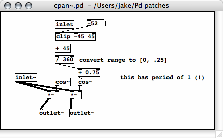
Hanning window, which is described by .5(1-cos(2*pi*t)) for t in [0,1].
This gave the grains a much smoother envelope.
Week Five
Monday: worked on my GS program, experimenting with
various controls on the grains. Trying to come up with a reliable way
of controlling the frequency range of the grains. My very crude
solution is to provide a "transposition" factor for each grain, which
simply scales the number of samples played in the fixed duration of the
grain. So for example, if transp = 1.5, and grain dur = 1000ms = 44100
samp, the final values for playing the grain will be 44100*1.5 samples
played in 1000ms. This actually turns out to control the percieved
freqency spread quite well, although of course it is relative to the
frequency content of the input material being granulated. Having an absolutely controlled freq. range would obviously require some tricky analysis of the grains. Update: I've changed the control units to octave transposition up and down.
Wednesday: Today I would like to think about analysis.
Yesterday afternoon I read a paper by Miller Puckette called
"Low-dimensional parameter mapping using spectral envelopes" (ICMC 2004
Proceedings). In the paper he describes a system for analyzing a live
input stream and mapping it to a parametrized curve in "timbre space",
some high dimensional vector space. There is also a library of
synthetic or stored and pre-analyzed sounds (though storing waveforms
for quick access will require a lot of memory). These sounds are also
assigned values in the same timbre space. In real time, the system then
synthesizes sound to match the live input. The simplest way of doing
this is, for each analysis interval to simply find the synthetic sound
with the minimum euclidean distance from the live input timbre.
Particularly valuable to think about right now are Puckette's
criteria for success. He mentions: (1) Perceptibility: changes in input
timbre should correspond to audible changes in output. (2) Robustness:
Slight variation in input shouldn't cause wild changes in output (and
the converse). (3) Continuity: Smoothly changing input shouldn't create
discontinuities in output. (4) Correspondence: When there is an audible
change in the input, the change in the output should be compatible
(softer->softer for example). (5) Fast response: musician must feel in control of the system.
I think that many of these apply in some way to our question of a RL
system using granular synthesized sounds as output and live audio as
input. At this point, I think it is an adequate challenge to use RL to
have a performer "teach" the GS to create a certain sort of texture. I
am still wondering whether it is necessary for the computer to be
granulating the actual audio input, or using it to control synthesis
parameters...
I also am going to look at doing some basic FFT analysis of the
granular output stream, with different window sizes. The idea is to use
this information for the RL state, consisting of a representation of
the frequency content of a recent timeframe of synthesized output. Then
maybe this information could be combined with/compared to a similar
windowed analysis of the live input signal to come up with a useful
ACTION. Some FFT based analysis techniques worth looking into seem to
be:
- spectral centroid: an amplitude weighted average of frequency bins, which corresponds to the preceptual brightness of the sound;
- A more general timbre-space representation like the one used by Puckette. He used his
[bonk~] object, which outputs strength of certain freqency bins. I'm going to look more into that.
Thursday:
Worked on my GS patch a lot. I don't really know
where to go with the RL thinking so I'm leaving it alone until next
week. I have turned my patch (currently called GranStretch) into
something very usable for composition/improvisation. I made several
examples yesterday of some possibilites. Most of them came after I
realized that there are great possibilities of input granulation by sequentially
moving the grain starting index through the buffer, rather than
constantly random positions being chosen. I stumbled across
pitch-preserving time stretching, which was exciting, I wasn't even
trying to create that ability. So a summary of the synth capabilities
is in order. There are essentially two parts; I'll start from the
lowest level:
- Grain generator. Current version is called
[oats2v~]> It is built to work with the nqpoly4
polyphonic voice manager patch. It accepts its parameters as a list in
the first inlet, and a bang on loading the abstraction (unused
currently). The parameter list is: grain start index (ms), grain
duration (ms), grain playback speed scaling (natural units), pan (from
-45 to 45 degrees) and source table number. Uses the [xplay~] object from Thomas Grill's xsample~
library. (Update: I have a version that just uses tabplay~ that works
just as well since I couldn't get xsample to work properly on my linux
machine.) Upon recieving a start time, throw~'s the grain audio
output to OUTL and OUTR summing busses. Has one outlet, which bangs
when the voice is done playing the current grain (which tells [nqpoly4] that the voice is free).
- Load.buffers: This provides eight buffers to load soundfiles into, they are named n-buf where n is the buffer number.
- Control: There are five sections for algorithmically generating
grain parameters. (These will eventually be partially or completely
taken over by the RL agent!) The control sections are as follows:
- grain.start.time: There is a rhythm subpatch which takes a
speed and deviation as params. It is basically a metronome which
imparts a randomized delay within the supplied deviation to each bang
it outputs. This can function as rhythmic variation when the speed is
sub-pitch, or begins to introduce noisiness if the speed is in the
pitch range and the grains are similar (a synchronous situation). This
is one of the most useful realtime performance controls. I'm thinking
about ways to increase its usability.
- grain.duration: generates a random duration between grain_dur_min and grain_dur_max.
One observation of mine that aligns with Curtis Roads' technique of
grainlets is that for a fixed grain length, lower pitched grains have a
clearer sense of pitch than higher grains. It seems like there might be
a better control than simply the length...something that takes into
account the pitch of the grain. Unfortunately that would be hard to
apply to granulation (no control over specific pitch of grains).
- grain.transposition: I talked about my method for grain transposition at the beginning of week five.
It is just simple time scaling; for example, if the transposition
factor is 2, twice as many samples are played from the buffer during
the given grain duration. To control this parameter I've set up two
horizontal sliders whose units are octaves, and control the upper and
lower bounds for transposition, respectively. The subpatch "makeTransp"
generates a transposition for each grain within this range and outputs
a corresponding scaling value for sending to the grain engine.
- grain.pick.buffers: Positive number n will cause random buffers between 1-buf and n-buf to be chosen. For n < 0, grains will only be taken from buffer |n|.
 grain.make.pan:
The pan for each grain is randomly generated within a distribution with
the mean set by the "pan" slider and the max. deviation set by the
"spread" number box. This uses the
grain.make.pan:
The pan for each grain is randomly generated within a distribution with
the mean set by the "pan" slider and the max. deviation set by the
"spread" number box. This uses the [pan~] external, which
accepts an angle in the range [-45,45] degrees. This is just constant
power panning, which I should code as an abstraction because I don't
know how standard the external is (I didn't have it on my linux
machine). (An abstraction is simply a Pd patch with inlets and
outlets, saved as a separate file. It can then be invoked the same way
an external is, as an object. The advantage over requiring an external
is that the abstraction can simply be packaged with the main patch,
without requiring a certain external to be installed [externals have to
be loaded at application start time].)
- Output: Putting a
[freeverb~] object at the output
adds some useful reverb possibilities (note: freeverb~ on linux doesn't
seem to work properly on my machine). The reverb tail "freeze" is a
neat effect. I've also set up a recording function using [sfwrite~] (note that this outputs a RAW sound file; I've been using the freeware program SoundHack to set the header information and save as AIFF).
Week Six
I uploaded the example pieces I made using my GranStretch patch last
week. Here they are, annotated. The source sounds for these came from the speech accent archive
at George Mason University. The description from their site: "This site
examines the accented [English] speech of speakers from many different
language backgrounds reading the same sample paragraph." These proved
to be interesting source material not only for the frequency variation
of the speech sounds, but also for the possibility of granulating
several of them in parallel, so grains of similar sounds appear
correlated in time in several of these examples.
- clickySpeedPiece:
This piece uses short grains, mostly on the order of less than 10ms. I
have found that grain durations in this range lose the identity of
their source completely, and so are useful in creating abstract
sounding clouds. Combined with high grain speeds, there is a variety of
familiar yet strange sounds available, from sawing and clicking to rich
gurgling and liquid sounds. Quickly varying the grain density yields
some very dramatic and useful transitions, the "evaporation" and
"condensation" of sounds. In this piece, several samples were being
simultaneously granulated, and the grain start pointer moved steadily
through the first ten seconds or so of the sound, over the course of
the minute and a half of sound. This technique makes use of the
transient consonants and longer vowels at a much slower time scale to
create movement in the frequency domain. In a sense, reading through
these speech samples took care of altering the grain frequency, which
one would have to control in synthetic GS.
- clickySpeedPiece2:
This piece is similar to the first, but I used the grain transposition
heavily, to achieve a wide range of frequency effects. This is where
the low gurgling and high rushing liquid noises start to shine. I also
pushed the grain durations into the 50-100 ms range in some places,
which illustrates how the grains start to contain the identity of their
sources at that length.
- voiceEvolve: This piece has grains read from a single sample, at a somewhat faster rate the that previous ones. There are also two
grain pointers moving linearly through the file at the same rate, but
from different starting points, in sort of a canon. The most apparent
characteristic is the much longer grain durations, in the range of a
few hundred milliseconds. This gives a strong pitch sense to the
grains, and you can identify the distinct vocal quality of the speaker.
There is no grain transposition, which also contributes to the
preservation of the voice's identity.
- groupMentality3 and groupMentality4:
These pieces use much longer grains, in the range of 1 - 1.5 seconds,
but maintaining a high grain density (with a grain repetition speed of
about 300-500ms). This creates enough grain overlap so that when only
one buffer is used, the original sound is completely preserved. In
these pieces, the only variation is changing the number of sample
buffers used. The first piece begins with only one sample then climaxes
to a full eight and back down to one. The second is more dense, and the
intelligibility of the speech disappears entirely, without losing the
clear identity of the voices; a very interesting effect.
We've been talking about using the analysis of an input audio signal
to create some sort of control stream for the granulation parameters.
For these experiments, we'll probably use some fixed sound material for
granulation, rather than using the live audio input itself in order to
simplify the experiment. Before we consider using RL to make granular
action decisions based on some audio input, we decided that it would be
good to see what we can do in terms of direct parameter mapping from
some parameters extracted from analysis.
I've also posted a few examples of grain clouds that I created using Curtis Roads's CloudGenerator
program, which can perform synthetic GS or granulation, asynchronous or
synchronous, with starting and ending values for frequency range, grain
duration, grain density, etc. I did these several weeks ago but they
are still somewhat instructive...
- clicks1.mp3: Synchronous short grains with increasing density. Begins to have a sense of pitch.
- clicks3.mp3: A continuation of the previous clip, with much higher density. Strong stable pitch sensation.
- clicks4.mp3: Same as clicks3 but the frequency in the grains begins to spread, making a hybrid pitched/noisy sensation.
- synch1.mp3: More synchronous short grains, with (I think) a constant frequency range, and increasing density.
- synch2.mp3: Same, but density ramps up to a higher value.
- synch4.mp3:
Same, but density goes MUCH higher. Here there is definitely a pitch
center to the noisy cloud, which comes from the synchronous repetition
of grains at a high speed. Each grain has a different frequency though
which makes the noisy component strong.
- synch5.mp3:
A synchronous cloud of sinusoidal grains with longer duration than the
previous ones. A fairly narrow frequency spread of grains.
- tone1.mp3:
Here is a steady tone, synchronous (?), long grains with a fast grain
speed (at the frequency of the tone). The stereo scattering of grains
gives it an interesting pulsing effect.
- tone2.mp3: Similar, but slower grain speeds, I think.
- myclicky.mp3:
This actually was made using my Pd patch, by using a buffer with a sine
wave being recorded into it. The frequency spread is due to both grain
transposition and a changing freqency sine wave being recording into
the buffer.
Week Seven
This week I focused more on the analysis end of things. The goal for
right now is just to come up with some useful analysis that will
produce a consistent control stream from some audio input (whether it's
a file or live audio input). I have been investigating the spectral centroid,
which I mentioned several weeks ago. It can be thought of as the
"center of gravity" of the spectrum in a certain finite frame of
analysis. It has been found to correspond to the intuitive "brightness"
of a sound. I've found it to be fairly easy to work with, although it
took me a while to realize how to implement it.
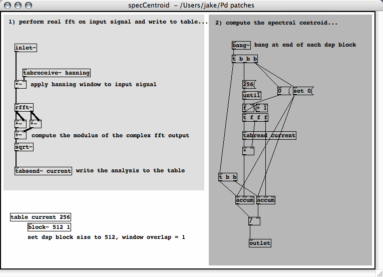
My implementation takes a signal input, applies a Hanning window to
it, then performs a real FFT. The modulus of the FFT output is taken
and written to an array (whose length is N/2 where N is the blocksize,
i.e. the window size of the analysis). I used the [bang~]
object, which sends out a bang at the end of each DSP cycle. The bang
triggers an iteration through the array and accumulates two sums, one
which is the dot product of a vector of FFT bin numbers and a vector of
their respective amplitudes, and the other which is the dot product of
the vector (1,1,...,1) and the amplitudes. A bang then divides the
first by the second and outputs the centroid of that frame. Here are
the screenshots:
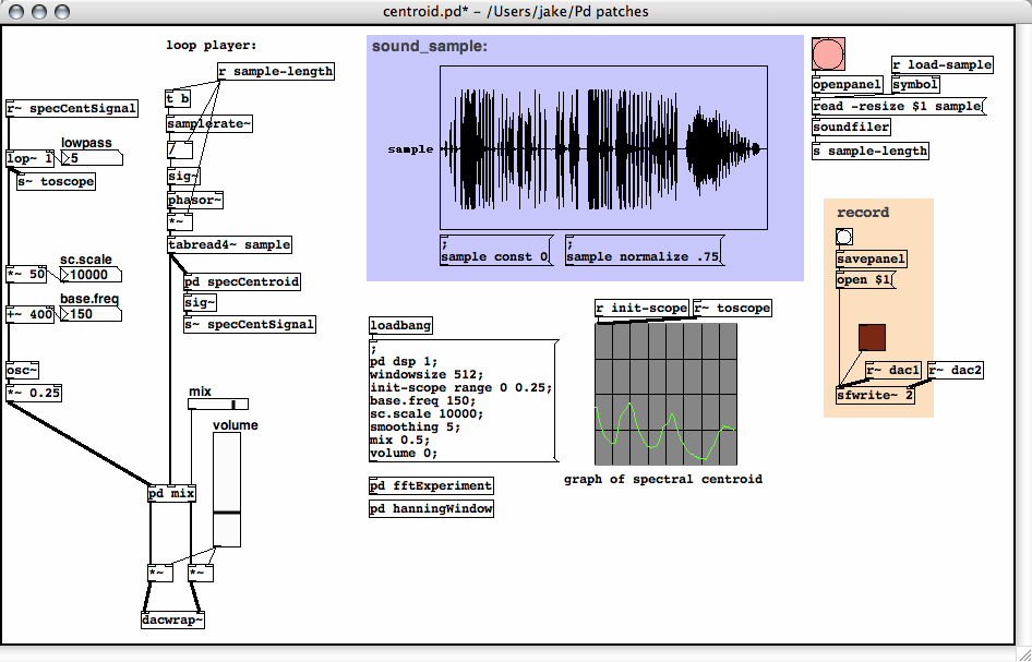
And a sonification (just a sine wave oscillator following the
centroid (which has been lowpassed to smooth it, and then scaled to an
appropriate frequency range): birdSpectralCentroid.mp3
I made a post
to the PD mailing list about other possible methods for feature
extraction.... The replies are definitely worth reading through. Some
of the statistical measures of the power spectrum could prove to be
useful. although I don't know anything about how the correlate to
perceived features in the audio.
Week Eight
Judy has started putting the reinforcement learning code into a flext
based external. I've been back into looking at flext, since Thomas
Grill has made some changes, most notably the new build system. I
tracked down the build system bug that was causing externals to compile
fine but then crash when loaded in PD. The thread is here: [PD] flext externals crash PD.
Friday: I'm looking at implementing some of the other spectral
measurements, namely I'm interested in calculating the variance and
standard deviation of the spectrum, using the spectral centroid as the
mean of the distribution. I think this will give some indication of the
"bandwidth" of the sound. I am sort of frustrated with programming this
kind of thing in PD; it ends up not being very elegant, the way it
makes you loop through an array and all. In search of a better
solution, I've been playing with Thomas Grill's py/pyext
externals. These let you quickly prototype PD external objects as
Python scripts. I'm completely new to Python but it seems like a very
simple, quick and clean language for doing this kind of thing. The
pyext Python module provides functions for getting data to and from
inlets and outlets, as well as accessing PD arrays and manipulating
them as arrays in Python (he uses the numarray module)!
Week Nine
We've decided on experimental setup that will be our work for the
rest of the summer. We've gotten Judy's flext port of the reinforcement
learning code working fairly well. The external is currently called [GrControl],
and implements the Sarsa-lambda algorithm for Sutton & Barto, based
on the implementation of another student of Judy's. I added flext
attribute functionality, so we can change the learning parameters on
the fly without recompiling the object.
Our thinking started with the pole-balancer task from the Sutton
& Barto's "Reinforcement Learning". This RL problem involves a cart
on a track which can move left and right, learning to balance a
vertical pole which is hinged to the cart. From the book:
The objective here is to apply forces to a cart moving along a track so
as to keep a pole hinged to the cart from falling over. A failure is
said to occur if the pole falls past a given angle from vertical or if
the cart reaches an end of the track. The pole is reset after each
failure. This task could be treated as episodic, where the natural
episodes are the repeated attempts to balance the pole. The reward in
this case could be +1 for every time step on which failure did not
occur, sos that the return at each time would be the number of steps
until failure....
The first mini-experiment with RL in Pure Data, superficially
similar to the pole-balancing problem, was to get the RL object to
learn a hidden rule (one particular desirable state). The states are
integers [0, 9]. The two possible actions are: increment the state by
one; or decrement the state by one. A reward of 0 is given when the
current state is the desired state (the hidden rule), and -1 is given
otherwise. Each time a reward of -1 is received, the RL algorithm
"fails" and begins a new episode, setting the state to a random value
and starting again.
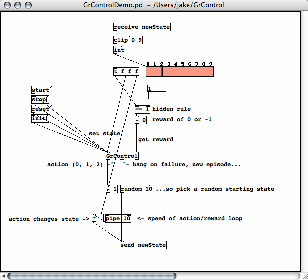
The second setup, shown below, uses the same states and actions, but
gives a reward of 1 upon hitting the target, and a reward of 0
otherwise. Upon getting a zero reward, the algorithm continues by
generating a new action. When a reward of 1 is received, the episode is
finished (so the actual reward "1" is used instead of the expected
reward from the algorithm's value function) but we still continue
generating actions. In summary, the state never gets reset to a random
starting value, making this more of a continuous learning setup.
The test setup looks like this:
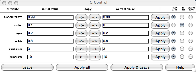
Below is the attributes dialog box, brought up by right-clicking on
GrControl and selecting "Properties". Here we can update the learning
parameters, which much be followed by an [init( message to the first inlet to actually update the params inside the algorithm. The [reset( message resets the Q values to random low values and clears the eligibility traces.
The next step will be to apply this to some audio output from the
granular synth patch ("Gran"). We decided it would be best to start out
with a very simple state space and actions space, similar to the
experiment above. The action space will be simply increasing or
decreasing the grain transposition setting in Gran. The states
will be read from a spectral centroid measurement of the granular
output. This seems to be a good choice since in my earlier experiments
I found the centroid to be strongly correlated to the transposition
setting (as one would expect). A positive (or zero) reward will be
given if the centroid at a given time step is within the desired range
of values. A negative reward will be given if the centroid at a given
time step is outside of that range. We hope that the RL program will be
able to find its way to the hidden rule of the desired centroid range,
and possibly that the learning process itself will generate interesting
musical material.
In order to have better control over the RL experiment, I created an
altered version of my Gran patch, called GranWave, which uses wavetable
oscillators to generate pure grains, rather than granulation
techniques. This is especially useful when I simply generate sine
grains, because I can set the grain transposition upper and lower
bounds to certain values, then actually expect the output to fall
within those ranges of the frequency spectrum (no harmonics to deal
with or anything). This works very well in practice, and will make it
possible to do much more controlled experiments.
I dicovered that my previous spectral centroid measurement
patch actually doesn't work properly (for whatever reason). I had a
hunch that it didn't, since it's measurement was sensitive to amplitude
changes in an otherwise constant sound input. I discovered that it is much simpler and cleaner to implement in Python using pyext.
Now I am confident that the measurement works properly. I've set up a
new spectral centroid visualization patch that shows the instantaneous
power spectrum with a range bar displaying the centroid right alongside
it. Feeding the input from GranWave into it, is is very satisfying to
watch the spectroid indicator consistently seek right to the visual as
well as aural center of the frequency distribution.
I also devised another power spectrum measurement that I'm calling
the "spread", which I also implemented in the same python script. I
wanted a measurement that would correspond to the "bandwidth" of the
grain cloud. At first I was thinking that a sort of "standard
deviation", using the centroid as the mean, would do it, but of course
that doesn't indicate the width of the spread around the centroid.
After thinking about it for a bit, I decided to try the following
calculation:
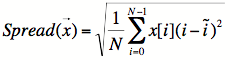
Where x = x0,...,xN-1 is the signal vector of length N, and i'
is the spectral centroid (in units of FFT bins). The idea was to use
the distance of each bin from the centroid bin, weighted by the
amplitude in that bin. This way, the more bins that are far away from
the centroid bin and have high amplitudes, the higher the total
measure will be. It turned out to be a good guess which correlates
quite well with the random transposition range of GranWave.
One thing to note about this "spread" measurement is that the way it is currently set up, the spread is linear
over the FFT bins, and therefore doesn't correspond well to what we
hear as the subjective pitch spread. I think it wouldn't be too hard to
change this to a "constant Q" spread that would give values that made
sense with respect to pitch rather than frequency. I think that might
be unnecessary complication for the experiment right now though, so I'm
going to stick with this frequency-linear version.
Week Ten
I'm working on applying our RL experiment setup to granular sound.
I'm planning on using 100 states, so first about that. There was a bit
of difficulty in getting the [GrControl] object to work with 100 states. I realized that I had to change a constant in RLControl.h:
#define MaxState 10 to
#define MaxState 100
Then it is just a matter of setting the numAgents attribute in the
GrControl object to 100, which you can do either with the "properties"
dialog box, or by creating the object as [GrControl @numAgents 100]
in which case that value is saved with the patch. When I had numAgents
exceeded MaxState, the code was generating some strange action values,
like constantly outputting "45", etc.
Next I found that if the actions are only +1,0,-1, a state space of
100 values is difficult to explore efficiently. I added two more
actions, +5 and -5, which allow for quicker exploration.
I'm going to use almost the same setup as we used in the simple "number finding" example (described in Week Nine).
The state will range in [0, 100]. Each state corresponds to a 220.5Hz
wide subband of the frequency spectrum. I am keeping it as linear
divisions of the spectrum for simplicity's sake, although it would be
more intuitive to divide it logarithmically.
Each signal block, the centroid is measured (in the GranAnalyze
patch). The GranRL patch receives that value and checks whether it is
within a certain range (settable by number boxes). If it is within the
range, a reward of "1" is sent, otherwise a reward of "0". The [GrControl]
object then first gets the state (the current setting of the
transposition control), followed by the reward. It outputs one of five
actions, which are adjustments of 0,+1,-1,+5,or -5 to the transposition
control. The process is then repeated.
When I got all this to work properly, it succeeded in finding the optimal setting fairly quickly.