MATLAB is a programming environment that runs on top of either Windows or Unix. Its syntax shares similarities with C, with some notable differences. It runs in an interactive mode, meaning that you can type single Matlab commands at a command prompt (a little bit like the Unix shell), and have them executed immediately. If you want, you may read more information on setting up your Matlab environment.
Matlab was originally designed for working efficiently with large matrices of numbers, and was adopted therefore by scientists and engineers. (A matrix is implemented as a two-dimensional array of numbers, but operations on matrices such as multiplication follow specific mathematical rules.) In this course, we'll use Matlab not so much for its abilities with matrices, but for the ease with which it handles and displays visual data (images and graphs). Of course, an image can also be seen as a matrix or set of matrices, as we will see.
Basics
Start Matlab up, and try the sequence of commands below. (Note: the >> is Matlab's command prompt, and is used to distinguish your commands from Matlab's responses.)
>> format compact
>> a = 7
a =
     7
>> b = [3 4]
b =
     3     4
>> c = [1 2; -1 0]
c =
     1     2
    -1     0
>> d = [b' c; b a];
>> d
d =
     3     1     2
     4    -1     0
     3     4     7
>>
The examples above create several variables using some of Matlab's basic data handling mechanisms. Notable points appear below:
- format compact suppresses extraneous line feeds, and is used to give a denser output.
- The first variable you created, a, has a single value (namely, 7). Such a variable is called a scalar. Matlab makes no distinction in storage between a scalar and an array or matrix: a scalar variable is treated as a 1x1 matrix, where the phrase "MxN matrix" by convention refers to a matrix with M rows and N columns. Matlab stores matrices in column-major order. (In other words, the elements of the first column are stored together in order, followed by the elements of the second column, etc.)
- The second variable you created, b, represents a vector of length
two, meaning that it has two independent components. In particular, b
is called a row vector, because the elements are arranged horizontally.
Again, Matlab makes no distinction between a row vector of length two and a 1x2
matrix. (Question: what kind of matrix would a column vector of length
two be?) You can check the dimensions of a variable using the length
and size functions.
>> length(b) ans = 2 >> size(b) ans = 1 2 >> - The third variable you created, c, represents a 2x2 matrix. Note that the components along each horizontal row are separated by either spaces or commas, and the rows are separated by semicolons.
 You don't have to build a matrix out of individual numbers -- larger blocks
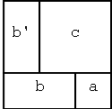
can be assembled also. The fourth variable you created, d, is built
up out of the smaller components already defined, to create a 3x3 matrix as
shown at right.
You don't have to build a matrix out of individual numbers -- larger blocks
can be assembled also. The fourth variable you created, d, is built
up out of the smaller components already defined, to create a 3x3 matrix as
shown at right.- The ' is a transpose operator, which flips matrices symmetrically around their diagonal axis. In the case of a row vector, the transpose converts it to a column vector, and vice versa.
- A semicolon at the end of a line suppresses the output of the result of that line. Thus d is not displayed initially as soon as it is created. To see it, we type its name without a semicolon.
Play with these methods of creating and displaying variables until you are comfortable with them.
Accessing Data
We've already seen how to print something out. But what if you want to print out (or perform some other operation on) only a part of some matrix or other data structure? Try the following sequence of commands.
>> b(2)
ans =
     4
>> d(2,2)
ans =
    -1
>> d(4)
ans =
     1
>> d([1 3],2)
ans =
     1
     4
>> d([1 3],[1 3])
ans =
     3     2
     3     7
>> d(3,[2 3]) = [10 10]
d =
     3     1     2
     4    -1     0
     3    10    10
>> d(4,4) = 7
d =
     3     1     2     0
     4    -1     0     0
     3    10    10     0
     0     0     0     7
>>
Again, these examples illustrate several important points:
- Matrices in Matlab are 1-indexed. In other words, the elements of b are numbered 1 and 2, not 0 and 1. This is a major difference from C and Java, and may be a source of confusion unless you are careful.
- Elements of a vector may be identified using a single index in parentheses.
- Elements of a matrix may be identified using two indices in parentheses.
- Elements of a matrix may also be identified using a single index in
parentheses, in which case the index refers to elements in column-major order.
The indices of the elements in d according to column-major order
appear below.
1 4 7 2 5 8 3 6 9 - Using a vector or matrix of indices yields a vector or matrix of elements
selected from the original matrix. Indices may even be repeated to build
results that are larger than the original:
>> d([1 2 3 1],[1 1 2 2 3 3]) ans = 3 3 1 1 2 2 4 4 -1 -1 0 0 3 3 4 4 7 7 3 3 1 1 2 2 >> - New values may be assigned to elements in a matrix using the = operator. Note that the size of the elements specified must match the dimensions of the new values provided. A 1x2 vector cannot fit into a 2x1 hole -- it must first be transposed using the ' operator.
- If a value is assigned to an element beyond the original size of a matrix, Matlab will expand it, filling in zeros for any new elements whose values are not specified. (Note that this may involve copying the old array, and so can be inefficient if done often. It's usually best to create the array in its ultimate size right from the start. This can be done using the zeros function, but we won't go into that now.)
Ranges of numbers
Often we will be interested in extracting a range of indices, or in creating a range of equally spaced numbers. The easiest way to do this is using the colon operator.
>> e = [1:6]
e =
     1     2     3     4     5     6
>> d(2:4,2:4)
ans =
    -1     0     0
    10    10     0
     0     0     7
>> d(:,2)
ans =
     1
    -1
    10
     0
>> d([1 2],:)
ans =
     3     1     2     0
     4    -1     0     0
>> c(:,:)
ans =
     1     2
    -1     0
>> d(end-1:end,2:end)
ans =
    10    10     0
     0     0     7
>> 1:.5:4
ans =
    1.0000    1.5000    2.0000    2.5000    3.0000    3.5000    4.0000
>> 7:-1:3
ans =
     7     6     5     4     3
>> linspace(0,1,5)
ans =
         0    0.2500    0.5000    0.7500    1.0000
>> linspace(0,1,6)
ans =
         0    0.2000    0.4000    0.6000    0.8000    1.0000
>>
Notable points:
- The expression a:b corresponds to a row vector of numbers from a to b, inclusive.
- Colon notation is commonly used to select a contiguous portion of an array.
- Within a matrix subscript reference, the colon used by itself indicates that the dimensions of the matrix itself should be used as bounds. Thus it is possible to automatically select an entire row, column, or set of rows or columns from an existing matrix.
- The special keyword end can be used to specify the upper limit of a selection using colon notation, based upon the size of the matrix in question. This is usually simpler and more clear than using the size function.
- Matrix indices must be integers. However, a:c:b colon notation can be used in other contexts to produce values that differ from one another by values other than 1.0. This is done by including the increment c as a third parameter between the two endpoints a and b.
- Another way to get ranges of equally spaced numbers is the linspace function. Instead of specifying the endpoints and the increment, you specify the endpoints and the total number of points, and let Matlab figure out the proper increment.
The colon operator can also be used to get different views of the shape of a particular data structure. For example, the following creates a 3-D array of random numbers, then views it in several ways. As a 3-D array, it is 5x3x2. As a 2D array, it is 5x6. As a vector, it is a column of length 30.
>> a = rand(5,3,2)
a(:,:,1) =
    0.9871    0.8040    0.6087
    0.8140    0.0885    0.4832
    0.5042    0.0512    0.1257
    0.4323    0.8353    0.2695
    0.9577    0.7497    0.0665
a(:,:,2) =
    0.7912    0.6061    0.5321
    0.7258    0.2604    0.5854
    0.9438    0.9831    0.1414
    0.0952    0.8842    0.0207
    0.3965    0.1726    0.1761
>> a(:,:)
ans =
    0.9871    0.8040    0.6087    0.7912    0.6061    0.5321
    0.8140    0.0885    0.4832    0.7258    0.2604    0.5854
    0.5042    0.0512    0.1257    0.9438    0.9831    0.1414
    0.4323    0.8353    0.2695    0.0952    0.8842    0.0207
    0.9577    0.7497    0.0665    0.3965    0.1726    0.1761
>> a(:)
ans =
    0.9871
    0.8140
    0.5042
    0.4323
    0.9577
    0.8040
    0.0885
    0.0512
    0.8353
    0.7497
    0.6087
    0.4832
    0.1257
    0.2695
    0.0665
    0.7912
    0.7258
    0.9438
    0.0952
    0.3965
    0.6061
    0.2604
    0.9831
    0.8842
    0.1726
    0.5321
    0.5854
    0.1414
    0.0207
    0.1761
>>
Loops
Loops in Matlab are simple to create, using the colon operator (or a preexisting row vector). However, they are usually not as fast as using a built-in function, because the built-in functions are heavily optimized. Below are some examples of using a loop. The functions tic and toc are used to time the commands. Note also the use of semicolons to separate several commands on the same line.
>> for i = 1:6
     d(i,i) = i;
   end
>> a = zeros(1,50000);
>> tic, for i = 1:50000, a(i) = i; end; toc
elapsed_time =
    0.1300
>> tic, a = [1:50000]; toc
elapsed_time =
     0
>>
Learning More
An important thing to learn about Matlab is how to learn more about a particular command or function. Matlab has an extensive library of built-in commands that do many useful things, and they are all well-described through the help system. (In fact, the hardest thing about using a Matlab command is often just being aware of its existence. You should learn to keep an eye out for the use of unfamiliar commands when you look at other peoples' code, as that's a good way of learning new tricks.)
As an example of how to learn more about a command, let's ask help to tell us more about a few things.
>> help linspace
>> help zeros
>> help diary
>> help help
You'll usually see a set of paragraphs describing how to use each command. Usually there are a couple of different ways to use each function, sometimes with examples. At the bottom is a list of related commands, which you can also learn about using help.
>> help lookfor
The lookfor command is another way to learn about Matlab, and is particularly useful if you know what you want to do but don't know any command that will do it.
Exercise
At this point, it's worth trying an exercise to apply some of what you have learned. We'll do this by creating some synthetic color images. Color images in Matlab are simply MxNx3 arrays. (N-dimensional arrays are handled similarly to 2-D matrices in terms of accessing their members. One way to construct a 3-D array is to build it up as a stack of 2-D planes, as shown below.)
>> f(:,:,1) = [1 3 5; 2 4 6];
>> f(:,:,2) = [7 9 11; 8 10 12];
>> f(:,:,3) = [13 15 17; 14 16 18];
>> f
f(:,:,1) =
     1     3     5
     2     4     6
f(:,:,2) =
     7     9    11
     8    10    12
f(:,:,3) =
    13    15    17
    14    16    18
>> imshow(f/18)
>>
The three planes of a color image represent the red, green, and blue components that make up each pixel in the image. All the values should range between zero and one. You can display an image on your screen using the imshow command. For example, the last line of the example above displays f as an image (after scaling it by a factor of 18 so that all the values range from 0 to 1). Since the largest values appear in the third plane, the image is dominated by blue. If the image is too small to see, you can blow it up via the somewhat cryptic command below. (Don't worry for now about what this is doing.)
>> set(gca,'Position',[0 0 1 1])
Your task is to create the images shown and described below. When you are finished, you should save them as .png files using the imwrite command, and turn in a transcript of the commands you used to create them. (You can create a transcript by copying from the Command History window and pasting into a text editor.)
- Image One
 This image is a 4x6x3 array (enlarged at right for visibility). Each column of
the image is a single color, in rainbow order. You'll need to experiment with
different combinations of red, green, and blue to get the look right. (Hint:
all the values in this image are either 0 or 1, except in the orange row where
one of the three color components is set to 0.5.)
This image is a 4x6x3 array (enlarged at right for visibility). Each column of
the image is a single color, in rainbow order. You'll need to experiment with
different combinations of red, green, and blue to get the look right. (Hint:
all the values in this image are either 0 or 1, except in the orange row where
one of the three color components is set to 0.5.)- Image Two
-
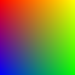 This 256x256 image contains gradations of color. The corners are
(clockwise from the top left) red, yellow, green, and blue. The intermediate
points are smoothly shaded from one end to the other. For example, the point at
the center top of the image is halfway between red and yellow (i.e., orange).
The point at the center bottom is halfway between blue and green (aqua), and
the point at the very center of the image is halfway between orange and aqua.
You could use loops to create this image, but it would be best if you can do
it without loops, using a few commands of colon notation.
This 256x256 image contains gradations of color. The corners are
(clockwise from the top left) red, yellow, green, and blue. The intermediate
points are smoothly shaded from one end to the other. For example, the point at
the center top of the image is halfway between red and yellow (i.e., orange).
The point at the center bottom is halfway between blue and green (aqua), and
the point at the very center of the image is halfway between orange and aqua.
You could use loops to create this image, but it would be best if you can do
it without loops, using a few commands of colon notation.