Special Studies in Computational Neuroscience Final Report, May 2018

Emma Jordan, Class of 2018

Advisor: Joseph O’Rourke

Introduction

The goal of this Special Studies was to serve as a capstone experience for the Computational Neuroscience student-designed major, by improving my understanding of machine learning and providing practical experience working with neural networks. Initially, I planned to conclude the semester by writing my own machine learning algorithm, but ended up adjusting the scope of the project to utilize an existing machine learning package instead, written in Python. Over the course of this project, I accomplished the following objectives:

1. Accumulate an understanding of current topics and ideas in computational neuroscience by reading relevant articles in the field
2. Select a pre-existing neuroscience-related dataset with accompanying paper and open-source Python code to a) understand and duplicate the results of and b) build on in some way.

The following report will describe my initial research, my processes of understanding and experimentation, and conclusions both regarding the paper and code I worked with and my original findings.

Preliminary research

Current research in computational neuroscience explores three main types of connections between neuroscience and machine learning. The first is using machine learning as a model of the human brain, either to learn how the brain works by looking at how ML algorithms work, or to improve ML algorithms by comparing them to how the brain works. One new program has been developed whose goal is to model small chunks (up to one cubic mm) of the human cortex by looking at activity in real brain slices (Singer 2016). Researchers in this program (Machine Intelligence from Cortical Networks, or “MICrONS”) take what they learn about the workings of the brain and apply it to creating improved neural networks. Some of these findings, to date, include general rules about cell wiring in the brain (cells that communicate with their own kind vs. cells avoiding their own kind) and an understanding of different possible models governing learning (learning based on knowledge of physics rules; building expectations for how things interact; forming expectations based on statistics).

MICrONS also utilizes machine learning in analysis of the data it gathers. This data is then able to inform neural networks and similar algorithms; for example, neural nets are now often written with feedback systems, a structure often observed in real brains (Singer 2016, Hassabis et. al. 2017). A few other brain mechanisms that have been incorporated into machine learning include visual processing based on attention and working memory buffers with central controllers, as well as the idea of episodic memory (Hassabis et. al. 2017). Memory is often encoded after repetition of information, but episodic memory describes a type of “one-shot” learning that scientists have recently found likely works due to “experience replay” during sleep. This finding can also be translated to neural networks by simulating repetition of high-priority information offline to promote learning. Additionally, researchers have found that our brains protect neurons against catastrophic forgetting, which we can apply to optimizing neural networks for new tasks without forgetting old ones (Hassabis et. al. 2017).

Research has also gone in the other direction: machine learning algorithms are helping to advance our understanding of the brain. By considering the brain’s functions in terms of machine-based concepts, we can gain more insight into its workings. Marblestone et. al. (2016) propose three such hypotheses about the brain: that it “optimizes cost functions”; that these cost functions are “diverse across areas and change over development”, and that “specialized systems allow efficient solution of key computational problems”. Proposals like these may help us experimentally learn more about the brain, stretching the way we think about it by comparing it to machine learning processes. New findings about how the brain works can then, in turn, be used to confirm the way we go about constructing machine learning algorithms and further improve them as well.

The second main connection between machine learning and neuroscience is through data analysis. With modern neuroscience and biology tools producing vast quantities of data, machine learning is more essential than ever to help distill meaning from all this information. It can be used in a variety of situations, from understanding biological systems to predicting drug effectiveness or medical diagnoses, and can help improve or even eliminate the shortcomings of human-generated models (Kording et. al. 2017). Machine learning is also now relatively easy to use, as pre-written algorithms are available on many platforms, and is better at making predictions about more complex, nonlinear data (Kording et. al. 2017).

Finally, machine learning can be used in direct interaction with brain signals, in the processes of neural decoding and encoding. Neural encoding relates neural signals to the external variables that may cause them, and neural decoding attempts to translate brain activity into corresponding intentions and physical actions (Kording et. al. 2017). One of the biggest application of neural decoding is neural control of prosthetic arms (Velliste et. al. 2008, Corbett et. al. 2012), as well as computer cursors or even actual muscles. To facilitate improvement of these applications, Glaser et. al. (2017) provide a benchmark of how standard decoding algorithms are doing in comparison to machine learning-based decoders, strong evidence that machine learning should become the new standard for neural decoding, and a comparison of several individual and ensemble machine learning algorithms. Since Glaser et. al.’s work is readily available online along with the datasets and full Python code used in their paper, I have chosen to work with their data and algorithms in my current project, with the following goals: to understand and replicate Glaser et. al.’s analyses, and to add to their findings through experimentation of my own with these algorithms.

“Machine Learning for Neural Decoding” paper and data

Data

Glaser et. al. (2017) use three main datasets in their research. The first two present data from motor and somatosensory cortex neurons of monkeys, and the velocity of their hand movements towards automated targets, recorded concurrently (Glaser et. al., 2018). The third dataset is similar, presenting recordings from hippocampus neurons in rats as well as their x and y coordinates as they follow rewards around a square platform (Mizuseki et. al. 2009). Hippocampal data is organized into three files, “spike times”, “pos”, and “pos times”. “Spike times” is an array of the hippocampal neurons recorded, each index of which contains an array of the timestamps at which that specific neuron spiked during the experiment. “Pos” and “pos times” contain information about the position of the rats in the open field: “pos times” is a vector of all recorded timestamps, and “pos” is a vector of the same length, with the xy coordinates of the rat’s head at each of those times. The S1 (somatosensory cortex) and M1 (motor cortex) datasets are organized similarly, but contain information about the x and y components of the velocity of the monkeys’ hand movements, as opposed to the x and y coordinates of the rats’ position. For the purposes of this project I will consider only the hippocampal and S1 datasets.

Code

The Python code that Glaser et. al. used in their paper, as well as example walkthroughs of formatting data and running it through their set of decoders, is available on Github (Glaser et. al. 2017). Downloaded data is initially in Matlab format, and first needs to be reformatted into Python as well as condensed into time bins of 0.2 seconds each. Formatted data is saved as two binned datasets: “neural_data”, which is a matrix of (time bins) x (number of neurons), where each entry is the average firing rate of a given neuron over a given time bin; and “pos_binned”, where each entry contains the average x and y position of the rat in each time bin.

        Formatted data can then be used to train and test any of the decoding algorithms included in the package. First, the user must select a range of neural data time bins around each output (position) that will be used to predict the output (in their example, the authors use 4 time bins of neural data before and after any given output). The “neural_data” matrix is then reformatted such that each time bin corresponds to both the spike information for that bin and the spike information for the appropriate number of previous and following bins. This new matrix is labelled “X” and will be the input matrix to each decoder. “Pos_binned” is relabelled “y” and will be the output information for decoding. Next, X and y are both split into training, testing, and validation sets. Each decoder algorithm can now be used to create a model using the training data, on which it will then base predictions about the output of the validation data. Finally, each decoder’s metric of fit (R2) is calculated by comparing output results from the model to the actual validation output. Glaser et. al. determine this fit separately for the x and y components of the position or velocity.

Paper

In their experimental study, Glaser et. al. compared the performance of eight neural network-based decoders, two linear regression-based decoders, and one ensemble model created from the predictions of most of the other decoders. Bayesian optimization was used to find the optimal hyperparameters (units, dropout, etc) for each decoder. They found that the machine learning decoders were significantly more powerful than the standard regression models, with the ensemble model making the best predictions overall. Neural networks were also much better at making predictions based on fewer input neurons, and appeared to withstand a range of changes to their hyperparameters. These findings suggest that, overall, neural networks are more suited to decoding than the current regression models.

Discrete Frechet Distance package

While following Glaser et. al.’s code and procedure to replicate the results of their decoders, I noticed that although both x and y position coordinates (in the hippocampal dataset; and x and y velocity components in the S1 dataset) were used to train each decoding model, they were considered separately while evaluating the metric of fit. For my own analyses, however, I decided to investigate whether the decoders could be evaluated more effectively by considering the xy position as a whole. My reasoning behind this was that, for the hippocampal dataset at least, the decoded output is in the form of the physical position of the moving rat, which depends on both x and y coordinates and relates both these components together in sequence. Therefore it was possible that neural data would be a better predictor of the position as a whole than of x and y position components individually. With this change, I also elected to use an additional metric of fit. With their Python package, Glaser et. al. provide functions to calculate the R2 and Pearson correlation values of decoder results. However, these values are typically used to measure the fit of a regression line, whereas I wanted to measure the closeness of two curves: the predicted and actual paths of the rat as it moved through the open field. For this purpose, I selected an additional Python package, “Discrete Frechet distance”, also available on Github. This package contains functions to calculate the Frechet distance, or the maximum distance between two comparable curves while moving along them at the same rate. Input to these functions consists of two 2-dimensional arrays of points.

Methods & Results

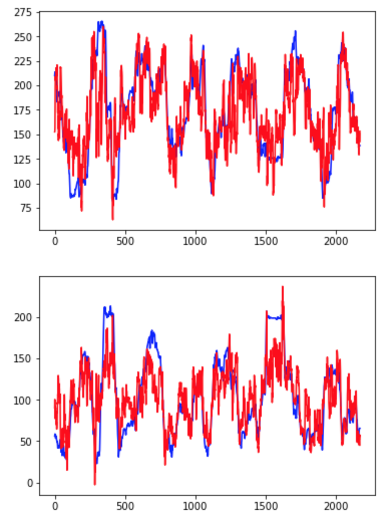
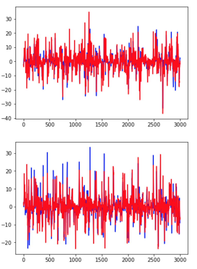
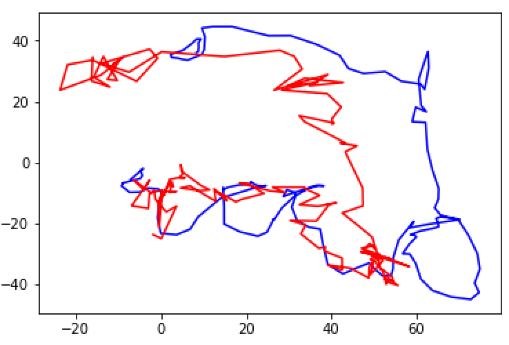
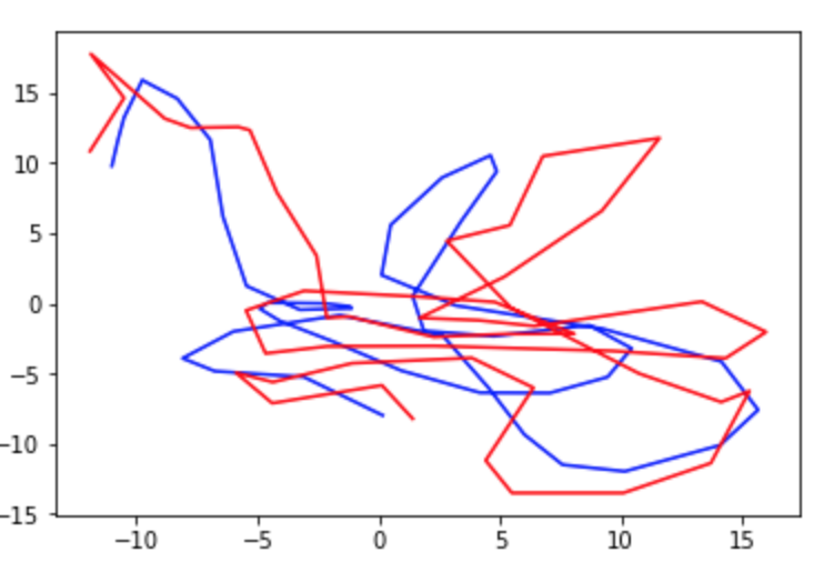
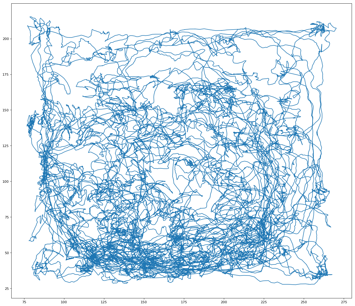
After completing the walkthrough included with Glaser et. al.’s code, I created several visualizations of the data. First, I used the original xy coordinates in the “pos” and “pos times” vectors to draw a line graph of the rat’s movements over the open field (Fig. 1). Next, I looked at the plots suggested in the walkthrough, which depict only changes in the rat’s x or y coordinate (Fig. 2) or the monkey’s x or y velocity (Fig. 3). These plots compare a 3000-time bin sample of actual output from the validation data to predicted output created using the Dense Neural Network (DNN) decoder. Next, I wanted to incorporate my addition of considering xy pairs as a whole, so I re-plotted the prediction graphs as continual paths (Figs 4 and 5). Since xy coordinates represented as a single path overlap a lot, I used much smaller samples (50 time bins each) to visualize the comparison. From these visualizations alone, it is clear that in general, the DNN was able to predict outputs in the S1 dataset more accurately than in the Hippocampal one, but its models are still fairly successful in both cases. Overall R2 values were calculated automatically for the entire dataset; in these initial runs, the Hippocampal DNN model came out at around R2 = 0.45 and the S1 DNN model at around R2 = 0.8.

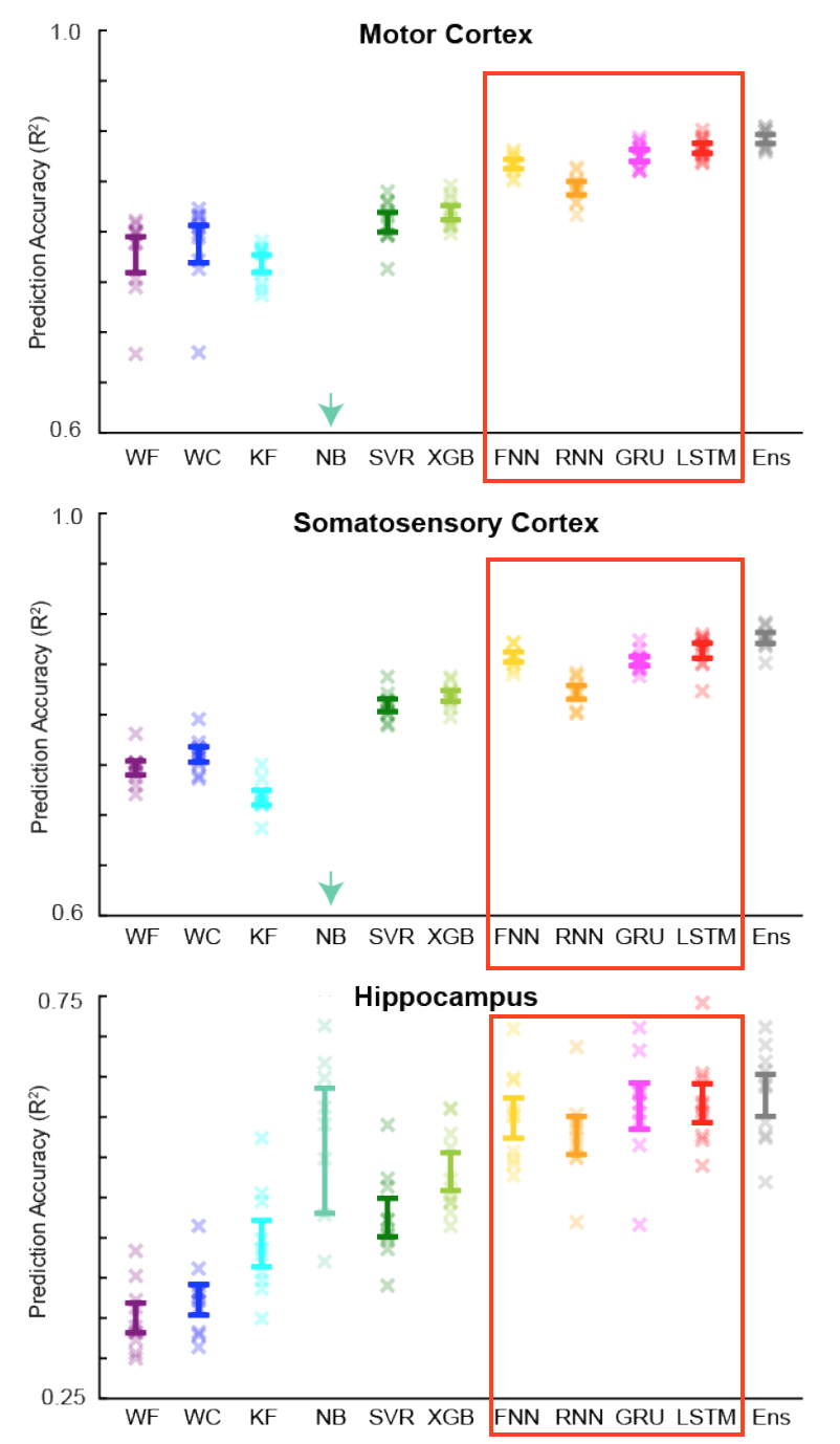
        Next, I took the code from Glaser et. al.’s decoder walkthrough and combined it with functions from the Frechet Distance package to create a pipeline that would take in one of the formatted datasets, use it to build a decoder model, and then produce statistics about the Frechet distance, Pearson correlation, and R2 values of the predicted vs. actual outputs. The algorithm to calculate Frechet distances between two curves works recursively, so it was not able to handle calculation of a 4000+ value dataset all at once. The algorithm also returns the greatest distance at any point between the input curves, whereas I was interested in learning the average distance between the actual and predicted curves overall. I got around both of these problems by continuing to sample the validation and predicted datasets in 50-time bin increments, calculating all three statistics (Frechet, Pearson, and R2) for each of these increments, and finally calculating the overall means, standard deviations, and medians of each statistic over the whole sampled dataset. I repeated this process over both the Hippocampal and the S1 datasets, and compared the performance of four of Glaser et. al.’s neural networks: the DNN, the Simple Recurrent Neural Network (RNN), the Long Short Term Memory Network (LSTM), and the Gated Recurrent Unit (GRU). Results are shown in Tables 1 and 2. For comparison, R2 results from the original paper are also included (Fig. 6). R2 results for the S1 dataset are comparable between this analysis and the original, while those for the Hippocampal dataset appear to be at least in similar proportions between neural networks, if not quite as accurate.

        Additionally, I experimented with changing the hyperparameters around on the various decoders I tested. For the S1 dataset, this did not seem to make much difference unless I set all the parameters very low (in which case predictions were very inaccurate); setting them much higher mainly resulted in my code taking longer to run. For the Hippocampal dataset, the suggested parameters (100 units, 25% dropout, and 10 epochs) did not produce sufficiently accurate predictions, so I increased DNN units to 2000 each on 40 layers. This improved results somewhat but still not to the level of the original results.

Fig. 1: Position of rat over time in the Hippocampal neuron dataset.

Fig. 2: Sample of Dense Neural Network predictions (shown in red) vs. actual values (shown in blue) of rats’ x (top graph) and y (bottom graph) coordinates over 3000 time bins.

Fig. 3: Sample of Dense Neural Network predictions (shown in red) vs. actual values (shown in blue) of monkeys’ x (top graph) and y (bottom graph) hand velocity components over 3000 time bins.

Fig. 4: Sample of DNN predictions (red) vs actual values (blue) of rats’ xy position over 50 time bins.

Fig. 5: Sample of DNN predictions (red) vs actual values (blue) of monkeys’ hand velocity over 50 time bins.

Table 1: Average Frechet distances, Pearson correlations, and R2 values for predicted vs. actual output from four neural networks for the Hippocampal and S1 datasets. Standard deviation values are included in parentheses.

Table 2: Median Frechet distances, Pearson correlations, and R2 values for predicted vs. actual output from four neural networks for the Hippocampal and S1 datasets.

Fig. 6: Part of Figure 4 from “Machine Learning for Neural Decoding” (Glaser et. al. 2017). R2 values are shown for all decoders, with error bars representing +/- SEM. The four neural networks used in the present analysis are highlighted with a red square.

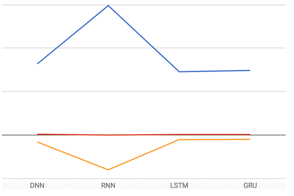
Fig. 7: Graphical representation of median Frechet distance (blue), median Pearson correlation (red), and media R2 (orange) for each decoder used on the Hippocampal dataset.

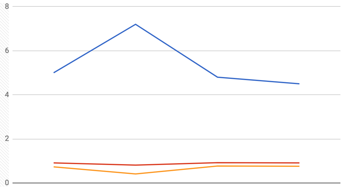
Fig. 8: Graphical representation of median Frechet distance (blue), median Pearson correlation (red), and median R2 (orange) for each decoder used on the S1 dataset.

Conclusions

Before starting this analysis, I hypothesized that using xy coordinates (as opposed to just x or y) as the output values of each neural network’s model would result in predictions at least as accurate, if not more so, than in Glaser et. al.’s original paper. I also thought that, in this case, the Frechet distance would be a better measure of how good each of these models were, since it is a measure of the closeness of two curves (or paths) as opposed to the closeness of regression lines. I generated two sets of statistics about the models I created: averages (Table 1) and medians (Table 2). When compared with results from the original paper, the medians from my analysis appear to be the more accurate of the two measures (possibly due to outliers), and within those, the neural networks were able to more accurately predict outputs in the S1 dataset than in the Hippocampal one. Median R2 values for the S1 dataset seem to be fairly close to those found by Glaser et. al. Median R2 values for the Hippocampal dataset are much lower than those in the original paper, but after accounting for this, they do follow the same trends when comparing across decoders: the LSTM and GRU networks are the best predictors, followed by the DNN, and the RNN is consistently the worst predictor of the four. These trends also appear consistently in the Pearson correlations and Frechet distances for both datasets. Figs. 7 and 8 show that the median Frechet distances follow roughly the inverse trend of the R2 values, which is about as expected and suggests that the Frechet distance is at least as good a measure of decoder model fit as R2 is.

        One thing I would change in a future iteration of this project would be to run the same Bayesian optimization method on the decoders’ hyperparameters that Glaser et. al. did in their paper code. I unfortunately did not have time to learn how to implement this optimization in my analysis, and instead just adjusted the parameters by hand until the neural networks’ performance improved slightly. I believe this is why the R2 values I got for all the neural networks trained on the Hippocampal dataset were so much lower than those in the original paper; parameter optimization would probably lead to more accurate results with this dataset. If I had more time I would also attempt to rewrite the machine learning functions used in the decoders with the Frechet distance directly incorporated into how they built their models instead of just used as a measure of fit after the fact. The Frechet distance could also be used in hyperparameter optimization. Finally, both this project and Glaser et. al.’s paper could be improved on by using a dataset of output information that is a little more directly relevant to neural control; although we have seen here that neural activity can predict the xy position of a rat fairly accurately, this is slightly arbitrary information, and it might be even better able to predict actions such as left vs. right movement.

References:

Corbett, E. A., Perreault, E. J., & Körding, K. P. (2012). Decoding with limited neural data: a mixture of time-warped trajectory models for directional reaches. Journal of neural engineering, 9(3), 036002.

Glaser, J. I., Chowdhury, R. H., Perich, M. G., Miller, L. E., & Kording, K. P. (2017). Machine learning for neural decoding. arXiv preprint arXiv:1708.00909.

Glaser J.I., Perich MG, Ramkumar P, Miller LE, Kording KP. (2018). Population Coding Of        Conditional Probability Distributions In Dorsal Premotor Cortex. bioRxiv. 2017:137026.

Hassabis, D., Kumaran, D., Summerfield, C., & Botvinick, M. (2017). Neuroscience-inspired artificial intelligence. Neuron, 95(2), 245-258.

Kording, K. P., Benjamin, A., Farhoodi, R., & Glaser, J. I. (2018, January). The Roles of Machine Learning in Biomedical Science. In Frontiers of Engineering: Reports on Leading-Edge Engineering from the 2017 Symposium. National Academies Press.

Marblestone, A. H., Wayne, G., & Kording, K. P. (2016). Toward an integration of deep learning and neuroscience. Frontiers in Computational Neuroscience, 10, 94.

Mizuseki K, Sirota A, Pastalkova E, Buzsáki G. (2009): Multi-unit recordings from the rat hippocampus made during open field foraging.
http://dx.doi.org/10.6080/K0Z60KZ9

Singer, E. (2016, April 6). Mapping the Brain to Build Better Machines. Quanta Magazine.

Velliste, M., Perel, S., Spalding, M. C., Whitford, A. S., & Schwartz, A. B. (2008). Cortical control of a prosthetic arm for self-feeding. Nature, 453(7198), 1098.