Today we'll be working with text data from several classic books available through Project Gutenberg:


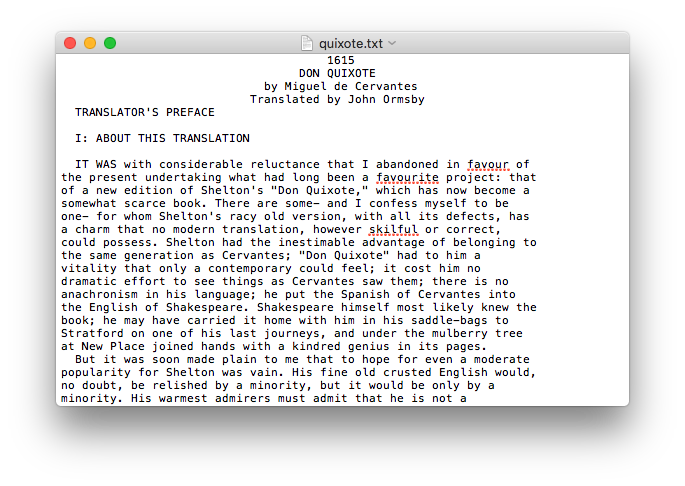
If we click on one of the titles above we, we can take a look at the raw text. For example, if we click Don Quixote, we get something that looks like this:
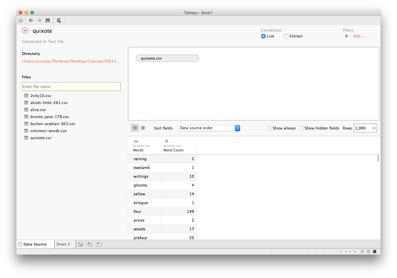
Unfortunately, raw text isn't very visualization-friendly without some preprocessing. I've written a quick script to process each book, and return a CSV file that contains each unique word that appears, along with its count. If you replace the .txt extension of any of the full text files with .csv, you'll be able to get these more manageable versions.
If we load one of these files into Tableau (I'll stick with Don Quixote, but feel free to use whichever book you like best!), we get something that looks like:
Let's pop over to a new sheet and see what we can do!
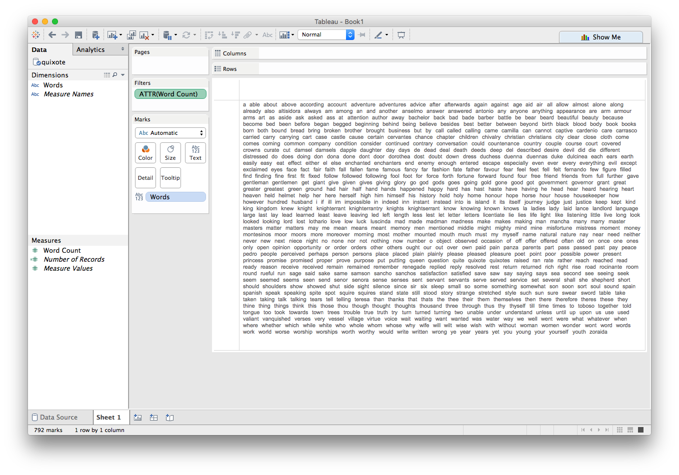
If we drag the Words dimension onto the Text mark, we can view all the unique words in the book:
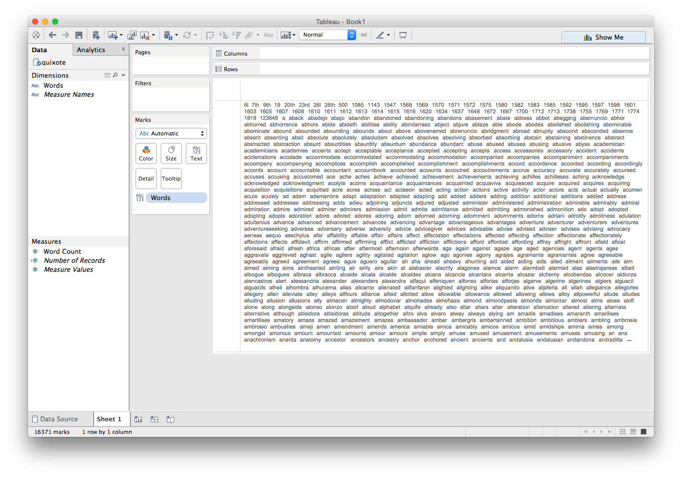
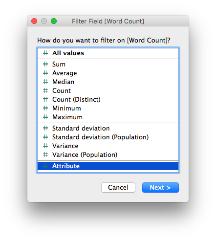
...well, almost. See how we only get partway through the As? There are too many unique words to fit! No problem, let's make a filter to show only those that appear at least 50 times:
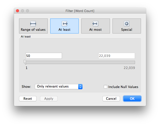
That's a little better:
Let's see what happens if we try using Word Count to drive the Size mark:
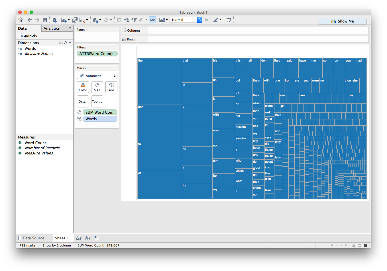
Ooh, sort of like a treemap!
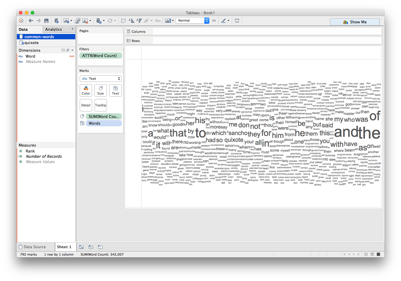
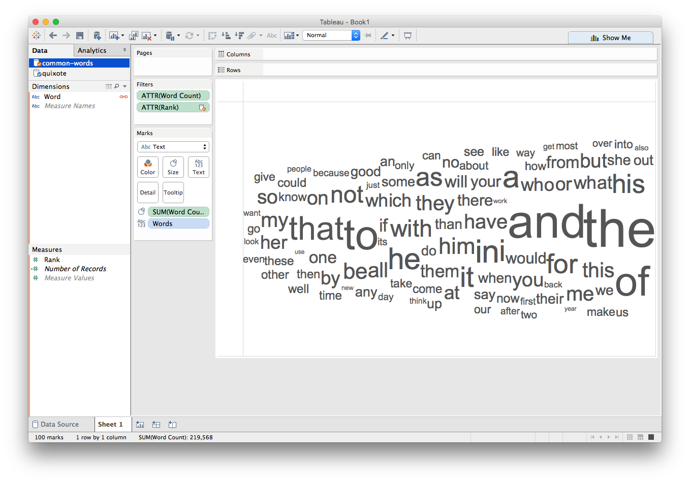
Let's switch from an Automatic mark type back to Text:
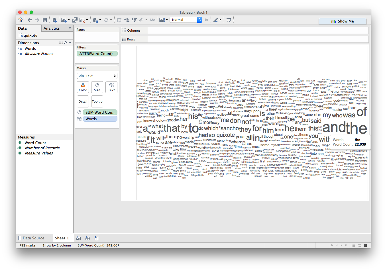
Hey, that's starting to look like a word cloud! There's just one problem: now that we've mapped Word Count to Size, it's easy to see that the most frequently used words aren't actually very informative.
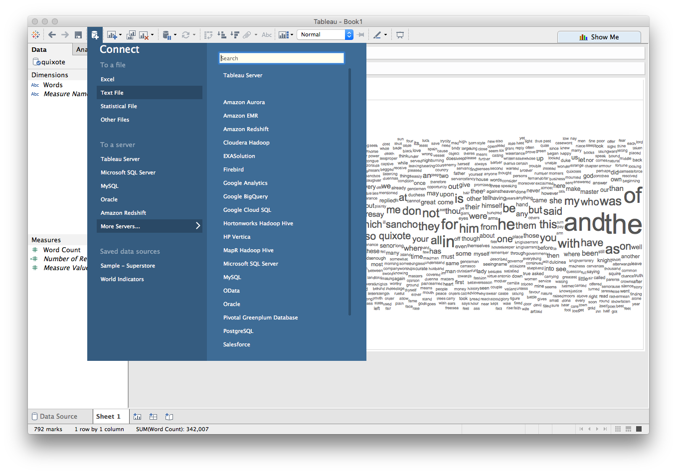
That's okay, we can filter again! This time, let's bring in a second data source that contains the 100 most commonly used English words. Start by clicking the Add a New Data Source... icon next to the Save button and select "Text File":
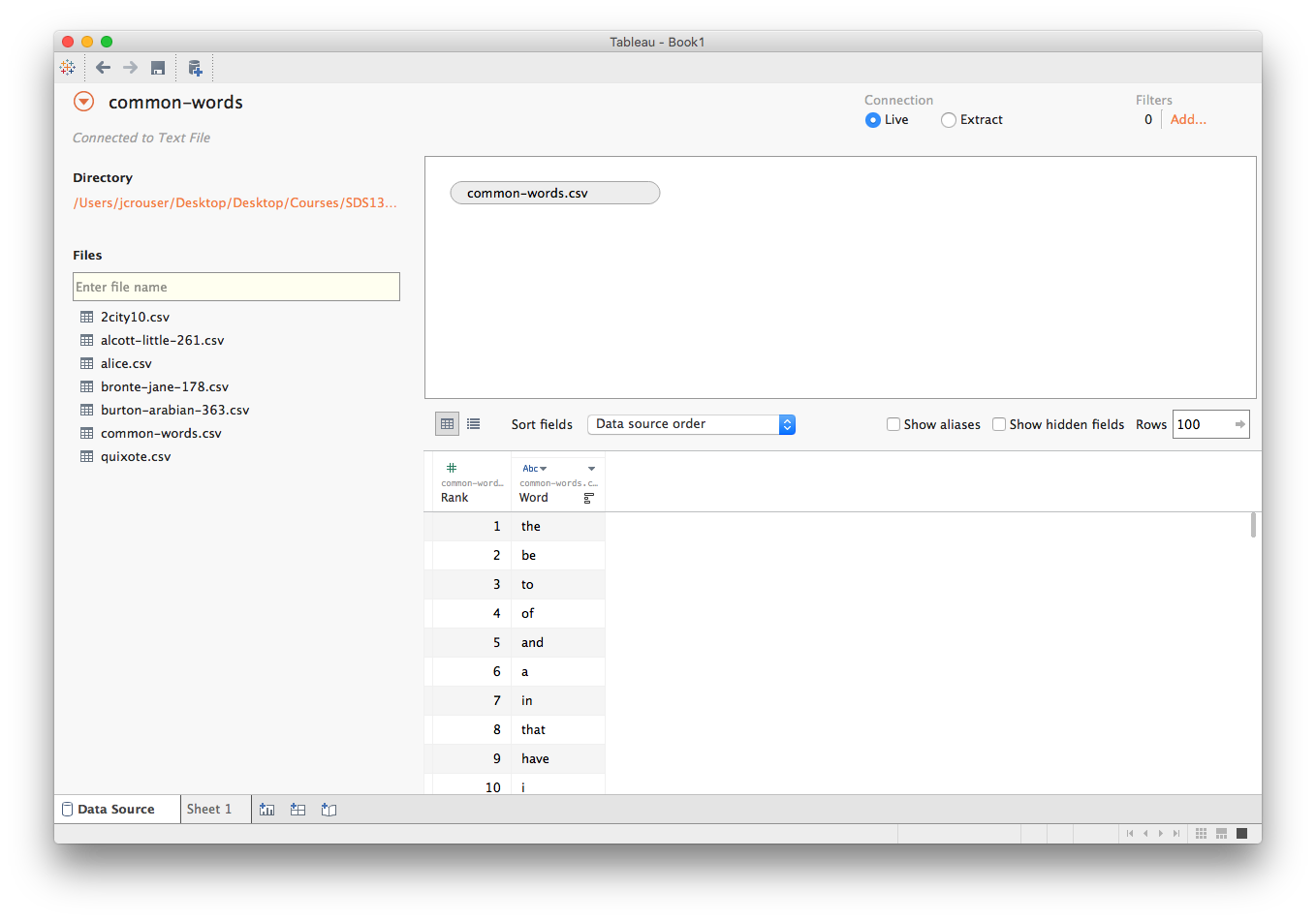
Now we'll connect to the common-words.csv file, which looks like this:
Now when wego backto the sheet, we should also see the second data source.
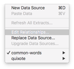
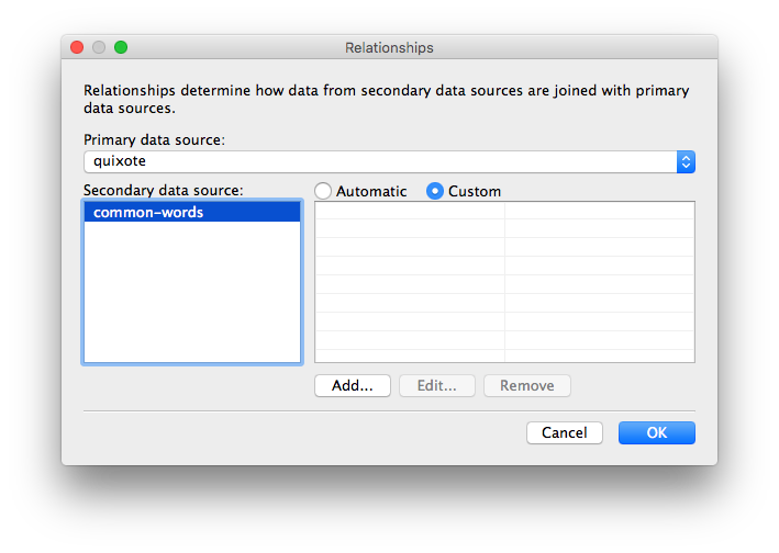
Before we'll be able to filter words in our book using words from this second file, we'll have to tell Tableau how to connect the two files. Start by selecting Edit Relationships... from the Data dropdown menu. In the following window, select the Custom radio button, and click Add...:
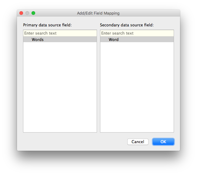
The only field they have in common is the Word field, so we can click OK:
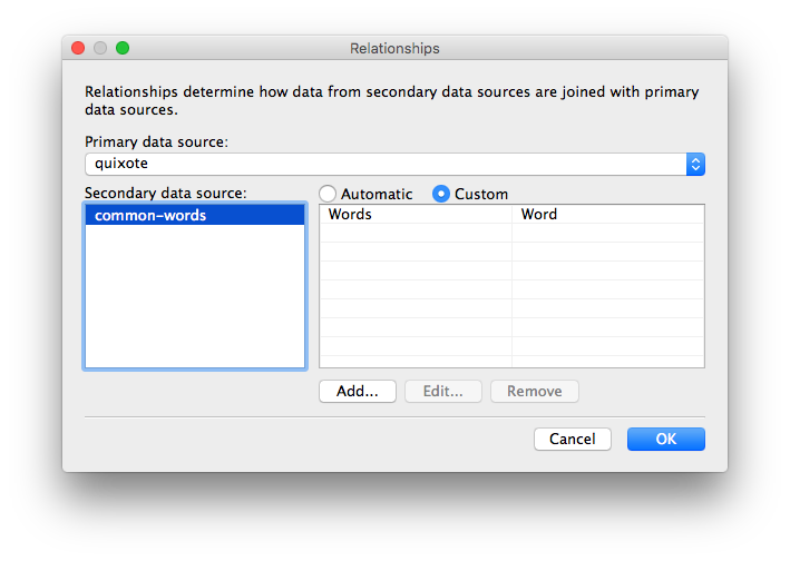
which will tell Tableau to connect these two fields, which will be indicated by a red link icon next to the Word dimension:
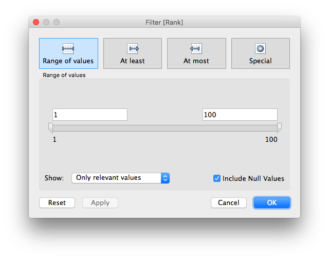
Now let's filter on Rank:
Uh oh! That's just the opposite of what we wanted.
Turns out that since the words we want to keep are the ones that don't appear in the common-words.csv file, we need to go back into our filter and tell Tableau to include null (or missing) values:
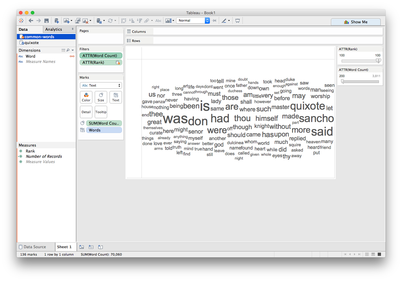
Now if we selectShow Filter for each of our filters, we can adjust how many of the most frequently used words to exclude, as well as set the threshold for how often a word has to appear in the book to be displayed. Here I've excluded all 100 most frequently used English words, and I'm only showing words that appear at least 200 times:
To make the larger words even more salient, we can use Color as a dual-encoding:
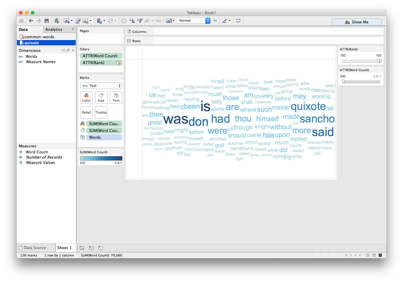
We can see that the names of the main characters (Don Quixote and Sancho) appear quite frequently!
Getting credit
Now it's your turn! To get credit for this lab, use your visualization to identify one interesting feature or trend in this dataset and post what you find to Piazza. You may want to try using this technique to compare two or more of the books to one another.